

x(t)
e
–αdx (t – t d )
d = Vt d
320
Biomedical Signal and Image Processing
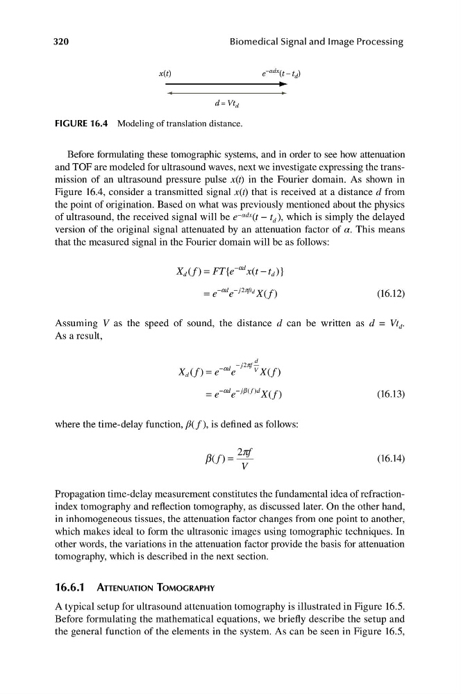
FIGURE 16.4 Modeling of translation distance.
Before formulating these tomographic systems, and in order to see how attenuation
and TOF are modeled for ultrasound waves, next we investigate expressing the transmission of an ultrasound pressure pulse x(t) in the Fourier domain. As shown in
Figure 16.4, consider a transmitted signal x(t) that is received at a distance d from
the point of origination. Based on what was previously mentioned about the physics
of ultrasound, the received signal will be e −αdx (t − t d ), which is simply the delayed
version of the original signal attenuated by an attenuation factor of α. This means
that the measured signal in the Fourier domain will be as follows:
X f
( ) = FT{e
−ad
d
x( t − t d )}
= e e
−ad − j 2pf t d X( )
f
(16.12)
Assuming V as the speed of sound, the distance d can be written as d = Vt d .
As a result,
d
− j f
2p
X f = e
−ad e
V
d ( )
X( )
f
= e e
− ad − jb ( )
f d X( )
f
(16.13)
where the time-delay function, β( f ), is defined as follows:
2pf
b( )
f =
(16.14)
V
Propagation time-delay measurement constitutes the fundamental idea of refractionindex tomography and reflection tomography, as discussed later. On the other hand,
in inhomogeneous tissues, the attenuation factor changes from one point to another,
which makes ideal to form the ultrasonic images using tomographic techniques. In
other words, the variations in the attenuation factor provide the basis for attenuation
tomography, which is described in the next section.
16.6.1 ATTENUATION TOMOGRAPHY
A typical setup for ultrasound attenuation tomography is illustrated in Figure 16.5.
Before formulating the mathematical equations, we briefly describe the setup and
the general function of the elements in the system. As can be seen in Figure 16.5,
e
–αdx (t – t d )
d = Vt d
320
Biomedical Signal and Image Processing
FIGURE 16.4 Modeling of translation distance.
Before formulating these tomographic systems, and in order to see how attenuation
and TOF are modeled for ultrasound waves, next we investigate expressing the transmission of an ultrasound pressure pulse x(t) in the Fourier domain. As shown in
Figure 16.4, consider a transmitted signal x(t) that is received at a distance d from
the point of origination. Based on what was previously mentioned about the physics
of ultrasound, the received signal will be e −αdx (t − t d ), which is simply the delayed
version of the original signal attenuated by an attenuation factor of α. This means
that the measured signal in the Fourier domain will be as follows:
X f
( ) = FT{e
−ad
d
x( t − t d )}
= e e
−ad − j 2pf t d X( )
f
(16.12)
Assuming V as the speed of sound, the distance d can be written as d = Vt d .
As a result,
d
− j f
2p
X f = e
−ad e
V
d ( )
X( )
f
= e e
− ad − jb ( )
f d X( )
f
(16.13)
where the time-delay function, β( f ), is defined as follows:
2pf
b( )
f =
(16.14)
V
Propagation time-delay measurement constitutes the fundamental idea of refractionindex tomography and reflection tomography, as discussed later. On the other hand,
in inhomogeneous tissues, the attenuation factor changes from one point to another,
which makes ideal to form the ultrasonic images using tomographic techniques. In
other words, the variations in the attenuation factor provide the basis for attenuation
tomography, which is described in the next section.
16.6.1 ATTENUATION TOMOGRAPHY
A typical setup for ultrasound attenuation tomography is illustrated in Figure 16.5.
Before formulating the mathematical equations, we briefly describe the setup and
the general function of the elements in the system. As can be seen in Figure 16.5,