

G z
G x
G y
FID
Echo
TE
TR
Time
90° RF
pulse
180° RF
pulse
294
Biomedical Signal and Image Processing
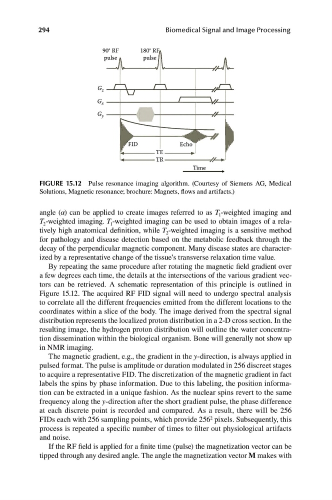
FIGURE 15.12 Pulse resonance imaging algorithm. (Courtesy of Siemens AG, Medical
Solutions, Magnetic resonance; brochure: Magnets, flows and artifacts.)
angle (α) can be applied to create images referred to as T 1 -weighted imaging and
T 2 -weighted imaging. T 1 -weighted imaging can be used to obtain images of a relatively high anatomical definition, while T 2 -weighted imaging is a sensitive method
for pathology and disease detection based on the metabolic feedback through the
decay of the perpendicular magnetic component. Many disease states are characterized by a representative change of the tissue’s transverse relaxation time value.
By repeating the same procedure after rotating the magnetic field gradient over
a few degrees each time, the details at the intersections of the various gradient vectors can be retrieved. A schematic representation of this principle is outlined in
Figure 15.12. The acquired RF FID signal will need to undergo spectral analysis
to correlate all the different frequencies emitted from the different locations to the
coordinates within a slice of the body. The image derived from the spectral signal
distribution represents the localized proton distribution in a 2-D cross section. In the
resulting image, the hydrogen proton distribution will outline the water concentration dissemination within the biological organism. Bone will generally not show up
in NMR imaging.
The magnetic gradient, e.g., the gradient in the y-direction, is always applied in
pulsed format. The pulse is amplitude or duration modulated in 256 discreet stages
to acquire a representative FID. The discretization of the magnetic gradient in fact
labels the spins by phase information. Due to this labeling, the position information can be extracted in a unique fashion. As the nuclear spins revert to the same
frequency along the y-direction after the short gradient pulse, the phase difference
at each discrete point is recorded and compared. As a result, there will be 256
FIDs each with 256 sampling points, which provide 256 2 pixels. Subsequently, this
process is repeated a specific number of times to filter out physiological artifacts
and noise.
If the RF field is applied for a finite time (pulse) the magnetization vector can be
tipped through any desired angle. The angle the magnetization vector M makes with
G x
G y
FID
Echo
TE
TR
Time
90° RF
pulse
180° RF
pulse
294
Biomedical Signal and Image Processing
FIGURE 15.12 Pulse resonance imaging algorithm. (Courtesy of Siemens AG, Medical
Solutions, Magnetic resonance; brochure: Magnets, flows and artifacts.)
angle (α) can be applied to create images referred to as T 1 -weighted imaging and
T 2 -weighted imaging. T 1 -weighted imaging can be used to obtain images of a relatively high anatomical definition, while T 2 -weighted imaging is a sensitive method
for pathology and disease detection based on the metabolic feedback through the
decay of the perpendicular magnetic component. Many disease states are characterized by a representative change of the tissue’s transverse relaxation time value.
By repeating the same procedure after rotating the magnetic field gradient over
a few degrees each time, the details at the intersections of the various gradient vectors can be retrieved. A schematic representation of this principle is outlined in
Figure 15.12. The acquired RF FID signal will need to undergo spectral analysis
to correlate all the different frequencies emitted from the different locations to the
coordinates within a slice of the body. The image derived from the spectral signal
distribution represents the localized proton distribution in a 2-D cross section. In the
resulting image, the hydrogen proton distribution will outline the water concentration dissemination within the biological organism. Bone will generally not show up
in NMR imaging.
The magnetic gradient, e.g., the gradient in the y-direction, is always applied in
pulsed format. The pulse is amplitude or duration modulated in 256 discreet stages
to acquire a representative FID. The discretization of the magnetic gradient in fact
labels the spins by phase information. Due to this labeling, the position information can be extracted in a unique fashion. As the nuclear spins revert to the same
frequency along the y-direction after the short gradient pulse, the phase difference
at each discrete point is recorded and compared. As a result, there will be 256
FIDs each with 256 sampling points, which provide 256 2 pixels. Subsequently, this
process is repeated a specific number of times to filter out physiological artifacts
and noise.
If the RF field is applied for a finite time (pulse) the magnetization vector can be
tipped through any desired angle. The angle the magnetization vector M makes with