

293
G x
FID
Time
G y
G z
90° Radio frequency pulse
Magnetic Resonance Imaging
Δf 4 Δf 3
Δz 3
Δz 4
z
Δz 2
Δz 1
Δf 2 Δf 1
f
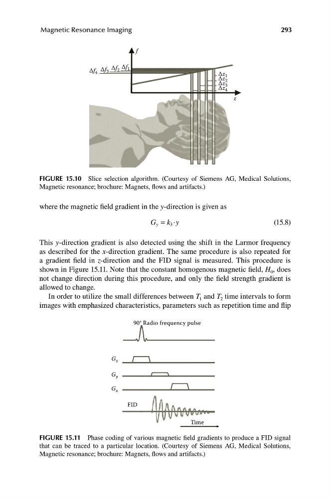
FIGURE 15.10 Slice selection algorithm. (Courtesy of Siemens AG, Medical Solutions,
Magnetic resonance; brochure: Magnets, flows and artifacts.)
where the magnetic field gradient in the y-direction is given as
.
G y = k 3 y
(15.8)
This y-direction gradient is also detected using the shift in the Larmor frequency
as described for the x-direction gradient. The same procedure is also repeated for
a gradient field in z-direction and the FID signal is measured. This procedure is
shown in Figure 15.11. Note that the constant homogenous magnetic field, H 0 , does
not change direction during this procedure, and only the field strength gradient is
allowed to change.
In order to utilize the small differences between T 1 and T 2 time intervals to form
images with emphasized characteristics, parameters such as repetition time and flip
FIGURE 15.11 Phase coding of various magnetic field gradients to produce a FID signal
that can be traced to a particular location. (Courtesy of Siemens AG, Medical Solutions,
Magnetic resonance; brochure: Magnets, flows and artifacts.)
G x
FID
Time
G y
G z
90° Radio frequency pulse
Magnetic Resonance Imaging
Δf 4 Δf 3
Δz 3
Δz 4
z
Δz 2
Δz 1
Δf 2 Δf 1
f
FIGURE 15.10 Slice selection algorithm. (Courtesy of Siemens AG, Medical Solutions,
Magnetic resonance; brochure: Magnets, flows and artifacts.)
where the magnetic field gradient in the y-direction is given as
.
G y = k 3 y
(15.8)
This y-direction gradient is also detected using the shift in the Larmor frequency
as described for the x-direction gradient. The same procedure is also repeated for
a gradient field in z-direction and the FID signal is measured. This procedure is
shown in Figure 15.11. Note that the constant homogenous magnetic field, H 0 , does
not change direction during this procedure, and only the field strength gradient is
allowed to change.
In order to utilize the small differences between T 1 and T 2 time intervals to form
images with emphasized characteristics, parameters such as repetition time and flip
FIGURE 15.11 Phase coding of various magnetic field gradients to produce a FID signal
that can be traced to a particular location. (Courtesy of Siemens AG, Medical Solutions,
Magnetic resonance; brochure: Magnets, flows and artifacts.)