

Principles of Computed Tomography
253
13.2 FORMULATION OF ATTENUATION
COMPUTED TOMOGRAPHY
In this section, a mathematical formulation of tomography is presented. In any tomographic system, a particular physical property of the tissue is used to generate an
image. For example, in attenuation tomography, the characteristics used to distinguish the points from each other, and therefore create an image based on these differences, is absorption index. In other words, if the absorption index of a point
(x, y) is shown by a 2-D function f(x, y), the tomographic image created will represent
the tissue based on the differences among the absorption index of each point inside
the tissue.
The main difficulty of almost all imaging systems is the fact that the value of the
function f(x, y) cannot be measured directly; rather, what is often measured is an integral in which f(x, y) acts as an integrand. In order to see this more clearly, let us examine
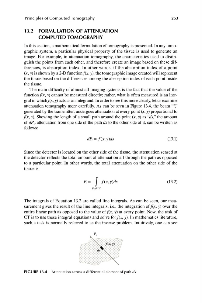
attenuation tomography more carefully. As can be seen in Figure 13.4, the beam “i,”
generated by the transmitter, undergoes attenuation at every point (x, y) proportional to
f(x, y). Showing the length of a small path around the point (x, y) as “ds,” the amount
of dP i , attenuation from one side of the path ds to the other side of it, can be written as
follows:
dP i = f x y ds
( , )
(13.1)
Since the detector is located on the other side of the tissue, the attenuation sensed at
the detector reflects the total amount of attenuation all through the path as opposed
to a particular point. In other words, the total attenuation on the other side of the
tissue is
P =
f xyd s
(13.2)
i
( , )
∫
Path i
“ ”
The integrals of Equation 13.2 are called line integrals. As can be seen, our measurement gives the result of the line integrals, i.e., the integration of f(x, y) over the
entire linear path as opposed to the value of f(x, y) at every point. Now, the task of
CT is to use these integral equations and solve for f(x, y). In mathematics literature,
such a task is normally referred to as the inverse problem. Intuitively, one can see
P i
ds
f (x, y)
FIGURE 13.4 Attenuation across a differential element of path ds.
253
13.2 FORMULATION OF ATTENUATION
COMPUTED TOMOGRAPHY
In this section, a mathematical formulation of tomography is presented. In any tomographic system, a particular physical property of the tissue is used to generate an
image. For example, in attenuation tomography, the characteristics used to distinguish the points from each other, and therefore create an image based on these differences, is absorption index. In other words, if the absorption index of a point
(x, y) is shown by a 2-D function f(x, y), the tomographic image created will represent
the tissue based on the differences among the absorption index of each point inside
the tissue.
The main difficulty of almost all imaging systems is the fact that the value of the
function f(x, y) cannot be measured directly; rather, what is often measured is an integral in which f(x, y) acts as an integrand. In order to see this more clearly, let us examine
attenuation tomography more carefully. As can be seen in Figure 13.4, the beam “i,”
generated by the transmitter, undergoes attenuation at every point (x, y) proportional to
f(x, y). Showing the length of a small path around the point (x, y) as “ds,” the amount
of dP i , attenuation from one side of the path ds to the other side of it, can be written as
follows:
dP i = f x y ds
( , )
(13.1)
Since the detector is located on the other side of the tissue, the attenuation sensed at
the detector reflects the total amount of attenuation all through the path as opposed
to a particular point. In other words, the total attenuation on the other side of the
tissue is
P =
f xyd s
(13.2)
i
( , )
∫
Path i
“ ”
The integrals of Equation 13.2 are called line integrals. As can be seen, our measurement gives the result of the line integrals, i.e., the integration of f(x, y) over the
entire linear path as opposed to the value of f(x, y) at every point. Now, the task of
CT is to use these integral equations and solve for f(x, y). In mathematics literature,
such a task is normally referred to as the inverse problem. Intuitively, one can see
P i
ds
f (x, y)
FIGURE 13.4 Attenuation across a differential element of path ds.