

112
Biomedical Signal and Image Processing
Autocorrelation
Time
Autocorrelation
Time
(a)
(b)
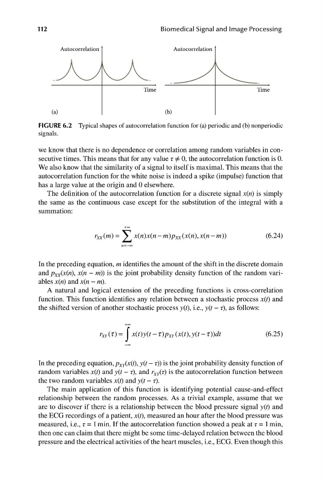
FIGURE 6.2 Typical shapes of autocorrelation function for (a) periodic and (b) nonperiodic
signals.
we know that there is no dependence or correlation among random variables in consecutive times. This means that for any value τ ≠ 0, the autocorrelation function is 0.
We also know that the similarity of a signal to itself is maximal. This means that the
autocorrelation function for the white noise is indeed a spike (impulse) function that
has a large value at the origin and 0 elsewhere.
The definition of the autocorrelation function for a discrete signal x(n) is simply
the same as the continuous case except for the substitution of the integral with a
summation:
+∞
r XX (m) =
x n x n
( ) ( − m p XX x n x n
)
( ( ), ( − m))
(6.24)
∑
n=−∞
In the preceding equation, m identifies the amount of the shift in the discrete domain
and p XX (x(n), x(n − m)) is the joint probability density function of the random variables x(n) and x(n − m).
A natural and logical extension of the preceding functions is cross-correlation
function. This function identifies any relation between a stochastic process x(t) and
the shifted version of another stochastic process y(t), i.e., y(t − τ), as follows:
+∞
r XY ( ) = xt yt − t ) p XY xt yt − t )) d t
t
( ) (
( ( ), (
(6.25)
∫
−∞
In the preceding equation, p XY (x(t), y(t − τ)) is the joint probability density function of
random variables x(t) and y(t − τ), and r XY (τ) is the autocorrelation function between
the two random variables x(t) and y(t − τ).
The main application of this function is identifying potential cause-and-effect
relationship between the random processes. As a trivial example, assume that we
are to discover if there is a relationship between the blood pressure signal y(t) and
the ECG recordings of a patient, x(t), measured an hour after the blood pressure was
measured, i.e., τ = 1 min. If the autocorrelation function showed a peak at τ = 1 min,
then one can claim that there might be some time-delayed relation between the blood
pressure and the electrical activities of the heart muscles, i.e., ECG. Even though this
Biomedical Signal and Image Processing
Autocorrelation
Time
Autocorrelation
Time
(a)
(b)
FIGURE 6.2 Typical shapes of autocorrelation function for (a) periodic and (b) nonperiodic
signals.
we know that there is no dependence or correlation among random variables in consecutive times. This means that for any value τ ≠ 0, the autocorrelation function is 0.
We also know that the similarity of a signal to itself is maximal. This means that the
autocorrelation function for the white noise is indeed a spike (impulse) function that
has a large value at the origin and 0 elsewhere.
The definition of the autocorrelation function for a discrete signal x(n) is simply
the same as the continuous case except for the substitution of the integral with a
summation:
+∞
r XX (m) =
x n x n
( ) ( − m p XX x n x n
)
( ( ), ( − m))
(6.24)
∑
n=−∞
In the preceding equation, m identifies the amount of the shift in the discrete domain
and p XX (x(n), x(n − m)) is the joint probability density function of the random variables x(n) and x(n − m).
A natural and logical extension of the preceding functions is cross-correlation
function. This function identifies any relation between a stochastic process x(t) and
the shifted version of another stochastic process y(t), i.e., y(t − τ), as follows:
+∞
r XY ( ) = xt yt − t ) p XY xt yt − t )) d t
t
( ) (
( ( ), (
(6.25)
∫
−∞
In the preceding equation, p XY (x(t), y(t − τ)) is the joint probability density function of
random variables x(t) and y(t − τ), and r XY (τ) is the autocorrelation function between
the two random variables x(t) and y(t − τ).
The main application of this function is identifying potential cause-and-effect
relationship between the random processes. As a trivial example, assume that we
are to discover if there is a relationship between the blood pressure signal y(t) and
the ECG recordings of a patient, x(t), measured an hour after the blood pressure was
measured, i.e., τ = 1 min. If the autocorrelation function showed a peak at τ = 1 min,
then one can claim that there might be some time-delayed relation between the blood
pressure and the electrical activities of the heart muscles, i.e., ECG. Even though this