

111
Other Signal and Image Processing Methods
assumption made in many biomedical signal and image processing applications,
and unless indicated otherwise, all stochastic processes discussed in the book are
assumed to be ergodic.
6.4.3 CORRELATION FUNCTIONS AND POWER SPECTRA
In order to express the time patterns within a stochastic signal as well as the interrelations across two or more stochastic signals, we need to have some practically useful measures and functions. For instance, since almost all biomedical signals have
some type of periodicity, it is extremely useful to explore such periodicities using
techniques such as Fourier transform (FT). However, since these signals are stochastic, we cannot simply apply FT to one only recording of the signal. The approach
we take in this section to address the aforementioned issue is rather simple; we construct meaningful determinist signals from a stochastic process and then process
these representative determinist signals using the FT and other techniques. As we
will see later in this chapter, these deterministic signals and measures are conceptually interesting and practically very meaningful. Even though the definition of these
signals and measures can be described for nonstationary processes too, due to the
fact that almost all biomedical applications processes and signals are assumed to
be stationary, we focus only on stationary processes and specialize all definitions
toward stationary processes.
The first function we discuss here is autocorrelation function. This function calculates the similarity of a signal to its shifted versions, i.e., it discovers the correlation
and similarity between x(t) and x(t − τ), where τ is the amount of shift. Specifically,
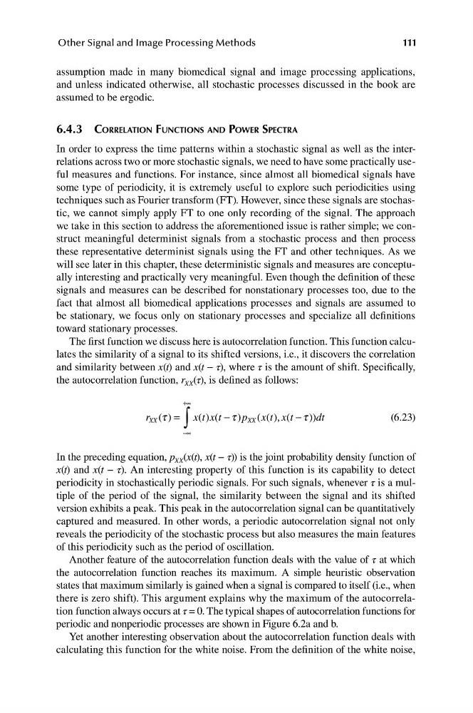
the autocorrelation function, r XX (τ), is defined as follows:
+∞
r ( ) = x t x t − t ) p x t x t − t )) dt
(6.23)
XX t
( ) (
XX ( ( ), (
∫
−∞
In the preceding equation, p XX (x(t), x(t − τ)) is the joint probability density function of
x(t) and x(t − τ). An interesting property of this function is its capability to detect
periodicity in stochastically periodic signals. For such signals, whenever τ is a multiple of the period of the signal, the similarity between the signal and its shifted
version exhibits a peak. This peak in the autocorrelation signal can be quantitatively
captured and measured. In other words, a periodic autocorrelation signal not only
reveals the periodicity of the stochastic process but also measures the main features
of this periodicity such as the period of oscillation.
Another feature of the autocorrelation function deals with the value of τ at which
the autocorrelation function reaches its maximum. A simple heuristic observation
states that maximum similarly is gained when a signal is compared to itself (i.e., when
there is zero shift). This argument explains why the maximum of the autocorrelation function always occurs at τ = 0. The typical shapes of autocorrelation functions for
periodic and nonperiodic processes are shown in Figure 6.2a and b.
Yet another interesting observation about the autocorrelation function deals with
calculating this function for the white noise. From the definition of the white noise,
Other Signal and Image Processing Methods
assumption made in many biomedical signal and image processing applications,
and unless indicated otherwise, all stochastic processes discussed in the book are
assumed to be ergodic.
6.4.3 CORRELATION FUNCTIONS AND POWER SPECTRA
In order to express the time patterns within a stochastic signal as well as the interrelations across two or more stochastic signals, we need to have some practically useful measures and functions. For instance, since almost all biomedical signals have
some type of periodicity, it is extremely useful to explore such periodicities using
techniques such as Fourier transform (FT). However, since these signals are stochastic, we cannot simply apply FT to one only recording of the signal. The approach
we take in this section to address the aforementioned issue is rather simple; we construct meaningful determinist signals from a stochastic process and then process
these representative determinist signals using the FT and other techniques. As we
will see later in this chapter, these deterministic signals and measures are conceptually interesting and practically very meaningful. Even though the definition of these
signals and measures can be described for nonstationary processes too, due to the
fact that almost all biomedical applications processes and signals are assumed to
be stationary, we focus only on stationary processes and specialize all definitions
toward stationary processes.
The first function we discuss here is autocorrelation function. This function calculates the similarity of a signal to its shifted versions, i.e., it discovers the correlation
and similarity between x(t) and x(t − τ), where τ is the amount of shift. Specifically,
the autocorrelation function, r XX (τ), is defined as follows:
+∞
r ( ) = x t x t − t ) p x t x t − t )) dt
(6.23)
XX t
( ) (
XX ( ( ), (
∫
−∞
In the preceding equation, p XX (x(t), x(t − τ)) is the joint probability density function of
x(t) and x(t − τ). An interesting property of this function is its capability to detect
periodicity in stochastically periodic signals. For such signals, whenever τ is a multiple of the period of the signal, the similarity between the signal and its shifted
version exhibits a peak. This peak in the autocorrelation signal can be quantitatively
captured and measured. In other words, a periodic autocorrelation signal not only
reveals the periodicity of the stochastic process but also measures the main features
of this periodicity such as the period of oscillation.
Another feature of the autocorrelation function deals with the value of τ at which
the autocorrelation function reaches its maximum. A simple heuristic observation
states that maximum similarly is gained when a signal is compared to itself (i.e., when
there is zero shift). This argument explains why the maximum of the autocorrelation function always occurs at τ = 0. The typical shapes of autocorrelation functions for
periodic and nonperiodic processes are shown in Figure 6.2a and b.
Yet another interesting observation about the autocorrelation function deals with
calculating this function for the white noise. From the definition of the white noise,