

92
Biomedical Signal and Image Processing
filter h(n). In reality, each choice of this filter results to one specific discrete mother
wavelet Ψ(n) according to the following iterative relations:
∑
N −1
Ψ ( )
n =
g(i ) Φ(2 n − i)
(5.13)
i= 0
where
( )
n = ∑
N −1
Φ
h(i ) Φ(2n − i)
(5.14)
i= 0
The function Φ(n) is often referred to as the “scaling function” and, in the previous
equation, helps the calculation of the mother wavelet. From the preceding equations, one can see that the mother wavelet of the operation is uniquely identified
and represented by the filter h(n) or, in other words, the role of the mother wavelet
is somehow replaced by h(n). The complexity of the iterative process of Equations
5.13 and 5.14, on the one hand, and the simple structure of the schematic diagram
of Figure 5.9, on the other hand, clearly state why in QMF algorithm one would
prefer to focus on the concept of h(n) as opposed to the direct use of the mother
wavelet. It can be shown that all popular discrete wavelets such as dbX can be
formed using QMF algorithm.
Another question, which is to the most part an open problem, is as follows: “How
many decomposition levels are needed for a suitable transform?” An intuitive
criterion to choose the level of the decomposition would be continuing decomposition until the highest known frequencies in the signal of interest are extracted and
identified. Loosely speaking, if one needs to have more detailed decomposition
of the signal in higher frequencies, he or she would need to calculate higher levels of
decomposition. This simply would allow more specific description of high-frequency
components of a signal.
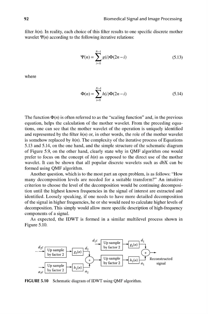
As expected, the IDWT is formed in a similar multilevel process shown in
Figure 5.10.
Up sample
by factor 2
d 2 c
a 2 c
...
Up sample
by factor 2
Up sample
by factor 2
g 1 (n)
Reconstructed
signal
h 1 (n)
g 1 (n)
a 1
d 1
d 1 c
a 2
+
d 2
+
Up sample
by factor 2
h 1 (n)
FIGURE 5.10 Schematic diagram of IDWT using QMF algorithm.
Biomedical Signal and Image Processing
filter h(n). In reality, each choice of this filter results to one specific discrete mother
wavelet Ψ(n) according to the following iterative relations:
∑
N −1
Ψ ( )
n =
g(i ) Φ(2 n − i)
(5.13)
i= 0
where
( )
n = ∑
N −1
Φ
h(i ) Φ(2n − i)
(5.14)
i= 0
The function Φ(n) is often referred to as the “scaling function” and, in the previous
equation, helps the calculation of the mother wavelet. From the preceding equations, one can see that the mother wavelet of the operation is uniquely identified
and represented by the filter h(n) or, in other words, the role of the mother wavelet
is somehow replaced by h(n). The complexity of the iterative process of Equations
5.13 and 5.14, on the one hand, and the simple structure of the schematic diagram
of Figure 5.9, on the other hand, clearly state why in QMF algorithm one would
prefer to focus on the concept of h(n) as opposed to the direct use of the mother
wavelet. It can be shown that all popular discrete wavelets such as dbX can be
formed using QMF algorithm.
Another question, which is to the most part an open problem, is as follows: “How
many decomposition levels are needed for a suitable transform?” An intuitive
criterion to choose the level of the decomposition would be continuing decomposition until the highest known frequencies in the signal of interest are extracted and
identified. Loosely speaking, if one needs to have more detailed decomposition
of the signal in higher frequencies, he or she would need to calculate higher levels of
decomposition. This simply would allow more specific description of high-frequency
components of a signal.
As expected, the IDWT is formed in a similar multilevel process shown in
Figure 5.10.
Up sample
by factor 2
d 2 c
a 2 c
...
Up sample
by factor 2
Up sample
by factor 2
g 1 (n)
Reconstructed
signal
h 1 (n)
g 1 (n)
a 1
d 1
d 1 c
a 2
+
d 2
+
Up sample
by factor 2
h 1 (n)
FIGURE 5.10 Schematic diagram of IDWT using QMF algorithm.