

91
Wavelet Transform
d 1 c
a 1 c
d 2 c
a 2 c
Down sample
by factor 2
Down sample
by factor 2
Down sample
by factor 2
Down sample
by factor 2
Input
signal
g(n)
h(n)
g(n)
h(n)
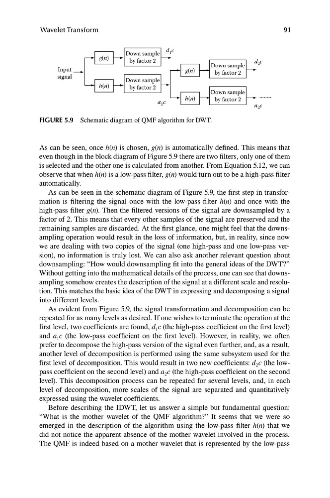
FIGURE 5.9 Schematic diagram of QMF algorithm for DWT.
As can be seen, once h(n) is chosen, g(n) is automatically defined. This means that
even though in the block diagram of Figure 5.9 there are two filters, only one of them
is selected and the other one is calculated from another. From Equation 5.12, we can
observe that when h(n) is a low-pass filter, g(n) would turn out to be a high-pass filter
automatically.
As can be seen in the schematic diagram of Figure 5.9, the first step in transformation is filtering the signal once with the low-pass filter h(n) and once with the
high-pass filter g(n). Then the filtered versions of the signal are downsampled by a
factor of 2. This means that every other samples of the signal are preserved and the
remaining samples are discarded. At the first glance, one might feel that the downsampling operation would result in the loss of information, but, in reality, since now
we are dealing with two copies of the signal (one high-pass and one low-pass version), no information is truly lost. We can also ask another relevant question about
downsampling: “How would downsampling fit into the general ideas of the DWT?”
Without getting into the mathematical details of the process, one can see that downsampling somehow creates the description of the signal at a different scale and resolution. This matches the basic idea of the DWT in expressing and decomposing a signal
into different levels.
As evident from Figure 5.9, the signal transformation and decomposition can be
repeated for as many levels as desired. If one wishes to terminate the operation at the
first level, two coefficients are found, d 1 c (the high-pass coefficient on the first level)
and a 1 c (the low-pass coefficient on the first level). However, in reality, we often
prefer to decompose the high-pass version of the signal even further, and, as a result,
another level of decomposition is performed using the same subsystem used for the
first level of decomposition. This would result in two new coefficients: d 2 c (the lowpass coefficient on the second level) and a 2 c (the high-pass coefficient on the second
level). This decomposition process can be repeated for several levels, and, in each
level of decomposition, more scales of the signal are separated and quantitatively
expressed using the wavelet coefficients.
Before describing the IDWT, let us answer a simple but fundamental question:
“What is the mother wavelet of the QMF algorithm?” It seems that we were so
emerged in the description of the algorithm using the low-pass filter h(n) that we
did not notice the apparent absence of the mother wavelet involved in the process.
The QMF is indeed based on a mother wavelet that is represented by the low-pass
Wavelet Transform
d 1 c
a 1 c
d 2 c
a 2 c
Down sample
by factor 2
Down sample
by factor 2
Down sample
by factor 2
Down sample
by factor 2
Input
signal
g(n)
h(n)
g(n)
h(n)
FIGURE 5.9 Schematic diagram of QMF algorithm for DWT.
As can be seen, once h(n) is chosen, g(n) is automatically defined. This means that
even though in the block diagram of Figure 5.9 there are two filters, only one of them
is selected and the other one is calculated from another. From Equation 5.12, we can
observe that when h(n) is a low-pass filter, g(n) would turn out to be a high-pass filter
automatically.
As can be seen in the schematic diagram of Figure 5.9, the first step in transformation is filtering the signal once with the low-pass filter h(n) and once with the
high-pass filter g(n). Then the filtered versions of the signal are downsampled by a
factor of 2. This means that every other samples of the signal are preserved and the
remaining samples are discarded. At the first glance, one might feel that the downsampling operation would result in the loss of information, but, in reality, since now
we are dealing with two copies of the signal (one high-pass and one low-pass version), no information is truly lost. We can also ask another relevant question about
downsampling: “How would downsampling fit into the general ideas of the DWT?”
Without getting into the mathematical details of the process, one can see that downsampling somehow creates the description of the signal at a different scale and resolution. This matches the basic idea of the DWT in expressing and decomposing a signal
into different levels.
As evident from Figure 5.9, the signal transformation and decomposition can be
repeated for as many levels as desired. If one wishes to terminate the operation at the
first level, two coefficients are found, d 1 c (the high-pass coefficient on the first level)
and a 1 c (the low-pass coefficient on the first level). However, in reality, we often
prefer to decompose the high-pass version of the signal even further, and, as a result,
another level of decomposition is performed using the same subsystem used for the
first level of decomposition. This would result in two new coefficients: d 2 c (the lowpass coefficient on the second level) and a 2 c (the high-pass coefficient on the second
level). This decomposition process can be repeated for several levels, and, in each
level of decomposition, more scales of the signal are separated and quantitatively
expressed using the wavelet coefficients.
Before describing the IDWT, let us answer a simple but fundamental question:
“What is the mother wavelet of the QMF algorithm?” It seems that we were so
emerged in the description of the algorithm using the low-pass filter h(n) that we
did not notice the apparent absence of the mother wavelet involved in the process.
The QMF is indeed based on a mother wavelet that is represented by the low-pass