

81
Wavelet Transform
Example 5.2
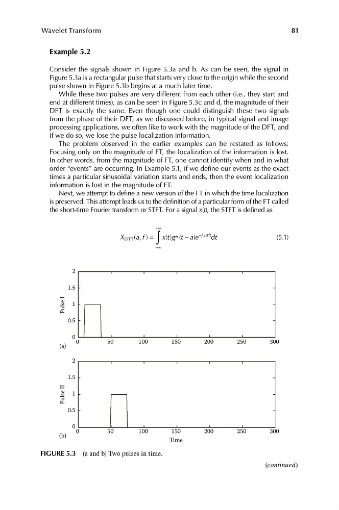
Consider the signals shown in Figure 5.3a and b. As can be seen, the signal in
Figure 5.3a is a rectangular pulse that starts very close to the origin while the second
pulse shown in Figure 5.3b begins at a much later time.
While these two pulses are very different from each other (i.e., they start and
end at different times), as can be seen in Figure 5.3c and d, the magnitude of their
DFT is exactly the same. Even though one could distinguish these two signals
from the phase of their DFT, as we discussed before, in typical signal and image
processing applications, we often like to work with the magnitude of the DFT, and
if we do so, we lose the pulse localization information.
The problem observed in the earlier examples can be restated as follows:
Focusing only on the magnitude of FT, the localization of the information is lost.
In other words, from the magnitude of FT, one cannot identify when and in what
order “events” are occurring. In Example 5.1, if we define our events as the exact
times a particular sinusoidal variation starts and ends, then the event localization
information is lost in the magnitude of FT.
Next, we attempt to define a new version of the FT in which the time localization
is preserved. This attempt leads us to the definition of a particular form of the FT called
the short-time Fourier transform or STFT. For a signal x(t), the STFT is defined as
+∞
X STFT ( ,
a f ) =
∫
x(t ) g ∗(t − a) e
−j 2pft dt
(5.1)
−∞
2
1.5
I
Pulse
1
0.5
0
0
50
100
150
200
250
300
(a)
2
1.5
II
Pulse
1
0.5
0
0
50
100
150
200
250
300
(b)
Time
FIGURE 5.3 (a and b) Two pulses in time.
(continued)
Wavelet Transform
Example 5.2
Consider the signals shown in Figure 5.3a and b. As can be seen, the signal in
Figure 5.3a is a rectangular pulse that starts very close to the origin while the second
pulse shown in Figure 5.3b begins at a much later time.
While these two pulses are very different from each other (i.e., they start and
end at different times), as can be seen in Figure 5.3c and d, the magnitude of their
DFT is exactly the same. Even though one could distinguish these two signals
from the phase of their DFT, as we discussed before, in typical signal and image
processing applications, we often like to work with the magnitude of the DFT, and
if we do so, we lose the pulse localization information.
The problem observed in the earlier examples can be restated as follows:
Focusing only on the magnitude of FT, the localization of the information is lost.
In other words, from the magnitude of FT, one cannot identify when and in what
order “events” are occurring. In Example 5.1, if we define our events as the exact
times a particular sinusoidal variation starts and ends, then the event localization
information is lost in the magnitude of FT.
Next, we attempt to define a new version of the FT in which the time localization
is preserved. This attempt leads us to the definition of a particular form of the FT called
the short-time Fourier transform or STFT. For a signal x(t), the STFT is defined as
+∞
X STFT ( ,
a f ) =
∫
x(t ) g ∗(t − a) e
−j 2pft dt
(5.1)
−∞
2
1.5
I
Pulse
1
0.5
0
0
50
100
150
200
250
300
(a)
2
1.5
II
Pulse
1
0.5
0
0
50
100
150
200
250
300
(b)
Time
FIGURE 5.3 (a and b) Two pulses in time.
(continued)