

3.2 Digital Implementation
63
y[n] = u[n] − x[n]
(3.5)
Where x[n] is the tracked slope baseline value and can be expressed as:
x[n] = x[n − 1] +
⎧
⎪ ⎨
⎪ ⎩
slope ↑
for u[n] > x[n − 1]
0
f o ru[n] = x[n − 1]
−slope ↓ for u[n] < x[n − 1]
(3.6a)
x[0] = u[0] (arbitrary)
(3.6b)
The filter has also a maximal slope, in the same sense as the BC2, but exceeding
the maximum slope only causes a time-limited deviation. As the filter does not have
acceptance thresholds, it also does not stay constant during an input pulse and as an
effect, the output pulse will be slightly affected.
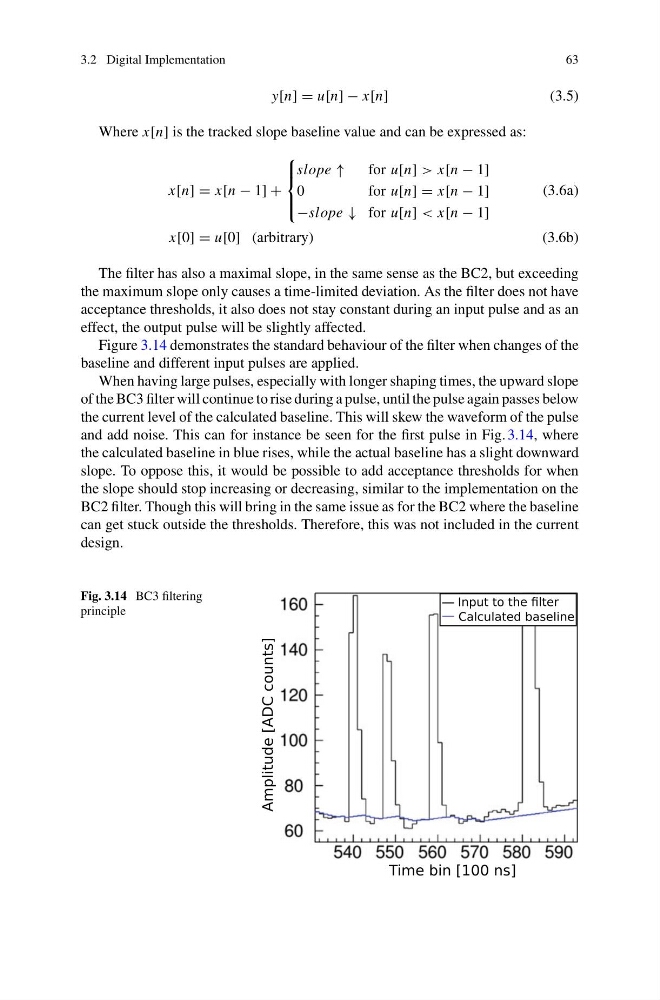
Figure 3.14 demonstrates the standard behaviour of the filter when changes of the
baseline and different input pulses are applied.
When having large pulses, especially with longer shaping times, the upward slope
of the BC3 filter will continue to rise during a pulse, until the pulse again passes below
the current level of the calculated baseline. This will skew the waveform of the pulse
and add noise. This can for instance be seen for the first pulse in Fig. 3.14, where
the calculated baseline in blue rises, while the actual baseline has a slight downward
slope. To oppose this, it would be possible to add acceptance thresholds for when
the slope should stop increasing or decreasing, similar to the implementation on the
BC2 filter. Though this will bring in the same issue as for the BC2 where the baseline
can get stuck outside the thresholds. Therefore, this was not included in the current
design.
Fig. 3.14 BC3 filtering
principle
63
y[n] = u[n] − x[n]
(3.5)
Where x[n] is the tracked slope baseline value and can be expressed as:
x[n] = x[n − 1] +
⎧
⎪ ⎨
⎪ ⎩
slope ↑
for u[n] > x[n − 1]
0
f o ru[n] = x[n − 1]
−slope ↓ for u[n] < x[n − 1]
(3.6a)
x[0] = u[0] (arbitrary)
(3.6b)
The filter has also a maximal slope, in the same sense as the BC2, but exceeding
the maximum slope only causes a time-limited deviation. As the filter does not have
acceptance thresholds, it also does not stay constant during an input pulse and as an
effect, the output pulse will be slightly affected.
Figure 3.14 demonstrates the standard behaviour of the filter when changes of the
baseline and different input pulses are applied.
When having large pulses, especially with longer shaping times, the upward slope
of the BC3 filter will continue to rise during a pulse, until the pulse again passes below
the current level of the calculated baseline. This will skew the waveform of the pulse
and add noise. This can for instance be seen for the first pulse in Fig. 3.14, where
the calculated baseline in blue rises, while the actual baseline has a slight downward
slope. To oppose this, it would be possible to add acceptance thresholds for when
the slope should stop increasing or decreasing, similar to the implementation on the
BC2 filter. Though this will bring in the same issue as for the BC2 where the baseline
can get stuck outside the thresholds. Therefore, this was not included in the current
design.
Fig. 3.14 BC3 filtering
principle