

E.2 Reliability
289
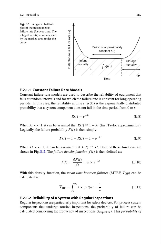
Fig. E.1 A typical bathtub
plot of the instantaneous
failure rate (λ) over time. The
integral of λ(t) is represented
by the marked area under the
curve
E.2.1.1 Constant Failure Rate Models
Constant failure rate models are used to describe the reliability of equipment that
fails at random intervals and for which the failure rate is constant for long operating
periods. In this case, the reliability at time t (R(t)) is the exponentially distributed
probability that a system component does not fail in the time period from 0 to t:
R(t) = e
−λt
(E.8)
When λt << 1, it can be assumed that R(t) ∼ = 1 − λt (first Taylor approximation).
Logically, the failure probability F (t) is then simply:
F (t) = 1 − R(t) = 1 − e
−λt
(E.9)
When λt << 1, it can be assumed that F (t) ∼ = λt. Both of these functions are
shown in Fig. E.2. The failure density function f (t) is then defined as:
f (t) =
dF (t)
dt
= λ × e
−λt
(E.10)
With this density function, the mean time between failures (MTBF, T BF ) can be
calculated as:
T BF =
∞
0
t × f (t)dt =
1
λ
(E.11)
E.2.1.2 Reliability of a System with Regular Inspections
Regular inspections are particularly important for safety devices. For process system
components that undergo routine inspections, the probability of failure can be
calculated considering the frequency of inspections (t inspection ). This probability of
289
Fig. E.1 A typical bathtub
plot of the instantaneous
failure rate (λ) over time. The
integral of λ(t) is represented
by the marked area under the
curve
E.2.1.1 Constant Failure Rate Models
Constant failure rate models are used to describe the reliability of equipment that
fails at random intervals and for which the failure rate is constant for long operating
periods. In this case, the reliability at time t (R(t)) is the exponentially distributed
probability that a system component does not fail in the time period from 0 to t:
R(t) = e
−λt
(E.8)
When λt << 1, it can be assumed that R(t) ∼ = 1 − λt (first Taylor approximation).
Logically, the failure probability F (t) is then simply:
F (t) = 1 − R(t) = 1 − e
−λt
(E.9)
When λt << 1, it can be assumed that F (t) ∼ = λt. Both of these functions are
shown in Fig. E.2. The failure density function f (t) is then defined as:
f (t) =
dF (t)
dt
= λ × e
−λt
(E.10)
With this density function, the mean time between failures (MTBF, T BF ) can be
calculated as:
T BF =
∞
0
t × f (t)dt =
1
λ
(E.11)
E.2.1.2 Reliability of a System with Regular Inspections
Regular inspections are particularly important for safety devices. For process system
components that undergo routine inspections, the probability of failure can be
calculated considering the frequency of inspections (t inspection ). This probability of