

252
10 Illustrative Case Study
10.4.2 Exposure Assessment (Step 2)
The second step of the assessment is to identify the level of exposure to ASM for the
environment and for humans (see Sect. 6.4). In this case study, the focus is placed on
(1) using an environmental fate model to predict the environmental exposure and (2)
using EFSA calculation tools to estimate both occupational and dietary consumer
exposure.
10.4.2.1 Environmental Exposure
In order to evaluate the fate of a chemical in the environment and to predict
the resulting environmental concentrations, environmental fate models can be
used. In these models, the environment is represented as a collection of wellmixed compartments (i.e., water, soil, and air), and the chemical concentration in
each compartment is calculated using partition coefficients and rate constants for
transport and transformation processes. Models can vary from level I to level IV,
which indicates the environmental processes included and the state of the system
considered in the model (see Sect. 6.4.2.2).
For the analysis of ASM, both level I and level III models available within
the small-world and small-region modeling tools will be used to investigate the
predicted environmental concentration (PEC) of ASM in the soil of an agricultural
field and in nearby water bodies. Both models are spreadsheet-based. The model file
and an introduction to using it are available online (Scheringer and MacLeod, 2021).
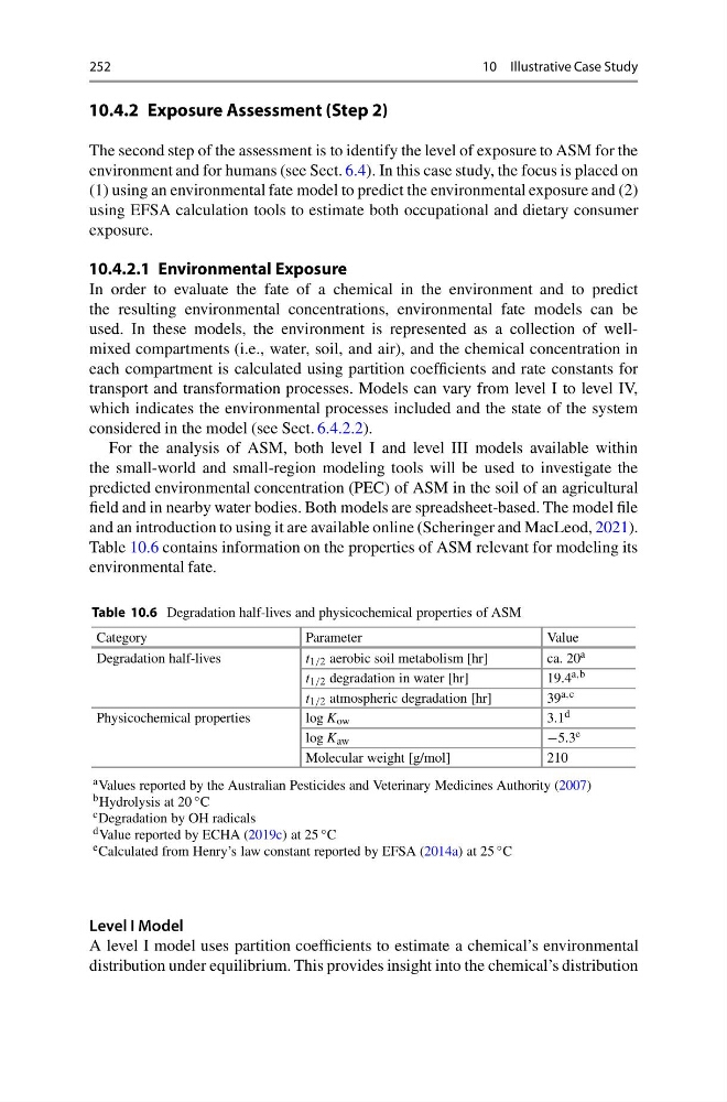
Table 10.6 contains information on the properties of ASM relevant for modeling its
environmental fate.
Table 10.6 Degradation half-lives and physicochemical properties of ASM
Category
Parameter
Value
Degradation half-lives
t 1/2 aerobic soil metabolism [hr]
ca. 20 a
t 1/2 degradation in water [hr]
19.4 a,b
t 1/2 atmospheric degradation [hr]
39 a,c
Physicochemical properties
log K ow
3.1 d
log K aw
−5.3 e
Molecular weight [g/mol]
210
a Values reported by the Australian Pesticides and Veterinary Medicines Authority (2007)
b Hydrolysis at 20 ◦ C
c Degradation by OH radicals
d Value reported by ECHA (2019c) at 25 ◦ C
e Calculated from Henry’s law constant reported by EFSA (2014a) at 25 ◦ C
Level I Model
A level I model uses partition coefficients to estimate a chemical’s environmental
distribution under equilibrium. This provides insight into the chemical’s distribution
10 Illustrative Case Study
10.4.2 Exposure Assessment (Step 2)
The second step of the assessment is to identify the level of exposure to ASM for the
environment and for humans (see Sect. 6.4). In this case study, the focus is placed on
(1) using an environmental fate model to predict the environmental exposure and (2)
using EFSA calculation tools to estimate both occupational and dietary consumer
exposure.
10.4.2.1 Environmental Exposure
In order to evaluate the fate of a chemical in the environment and to predict
the resulting environmental concentrations, environmental fate models can be
used. In these models, the environment is represented as a collection of wellmixed compartments (i.e., water, soil, and air), and the chemical concentration in
each compartment is calculated using partition coefficients and rate constants for
transport and transformation processes. Models can vary from level I to level IV,
which indicates the environmental processes included and the state of the system
considered in the model (see Sect. 6.4.2.2).
For the analysis of ASM, both level I and level III models available within
the small-world and small-region modeling tools will be used to investigate the
predicted environmental concentration (PEC) of ASM in the soil of an agricultural
field and in nearby water bodies. Both models are spreadsheet-based. The model file
and an introduction to using it are available online (Scheringer and MacLeod, 2021).
Table 10.6 contains information on the properties of ASM relevant for modeling its
environmental fate.
Table 10.6 Degradation half-lives and physicochemical properties of ASM
Category
Parameter
Value
Degradation half-lives
t 1/2 aerobic soil metabolism [hr]
ca. 20 a
t 1/2 degradation in water [hr]
19.4 a,b
t 1/2 atmospheric degradation [hr]
39 a,c
Physicochemical properties
log K ow
3.1 d
log K aw
−5.3 e
Molecular weight [g/mol]
210
a Values reported by the Australian Pesticides and Veterinary Medicines Authority (2007)
b Hydrolysis at 20 ◦ C
c Degradation by OH radicals
d Value reported by ECHA (2019c) at 25 ◦ C
e Calculated from Henry’s law constant reported by EFSA (2014a) at 25 ◦ C
Level I Model
A level I model uses partition coefficients to estimate a chemical’s environmental
distribution under equilibrium. This provides insight into the chemical’s distribution