

traveling with speed v and mass m 0 ¼ 9:11 Â 10
À31 kg at v ¼ 0 (“rest mass”) is
calculated by:
m ¼
m 0
1 À
v
c
h
i 1
2
ð12:23Þ
where c ¼ 2:998 Â 10
8 ms
À1 is the speed of light. After inserting in Eq. (12.21), one
obtains:
l ¼
h
2m 0 eV 1 þ
eV
2m 0 c 2
! 1
2
ð12:24Þ
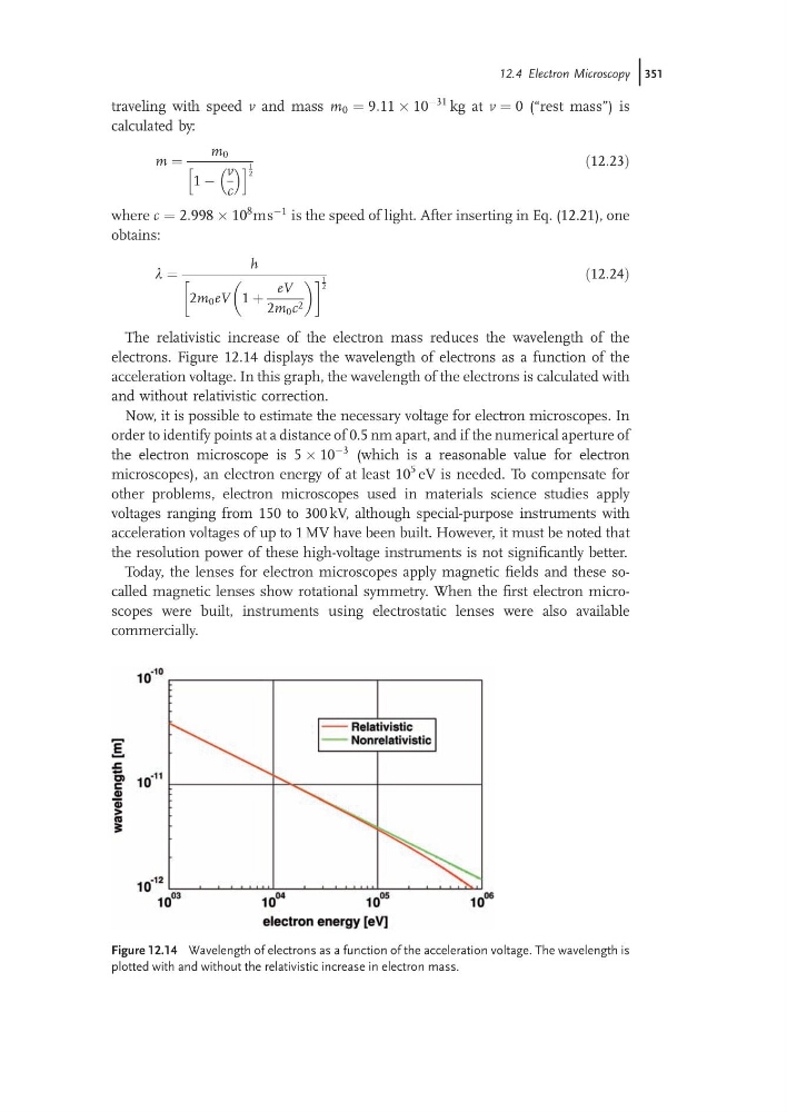
The relativistic increase of the electron mass reduces the wavelength of the
electrons. Figure 12.14 displays the wavelength of electrons as a function of the
acceleration voltage. In this graph, the wavelength of the electrons is calculated with
and without relativistic correction.
Now, it is possible to estimate the necessary voltage for electron microscopes. In
order to identify points at a distance of 0.5 nm apart, and if the numerical aperture of
the electron microscope is 5 Â 10
À3 (which is a reasonable value for electron
microscopes), an electron energy of at least 10
5 eV is needed. To compensate for
other problems, electron microscopes used in materials science studies apply
voltages ranging from 150 to 300 kV, although special-purpose instruments with
acceleration voltages of up to 1 MV have been built. However, it must be noted that
the resolution power of these high-voltage instruments is not significantly better.
Today, the lenses for electron microscopes apply magnetic fields and these socalled magnetic lenses show rotational symmetry. When the first electron microscopes were built, instruments using electrostatic lenses were also available
commercially.
Figure 12.14 Wavelength of electrons as a function of the acceleration voltage. The wavelength is
plotted with and without the relativistic increase in electron mass.
12.4 Electron Microscopy j351
À31 kg at v ¼ 0 (“rest mass”) is
calculated by:
m ¼
m 0
1 À
v
c
h
i 1
2
ð12:23Þ
where c ¼ 2:998 Â 10
8 ms
À1 is the speed of light. After inserting in Eq. (12.21), one
obtains:
l ¼
h
2m 0 eV 1 þ
eV
2m 0 c 2
! 1
2
ð12:24Þ
The relativistic increase of the electron mass reduces the wavelength of the
electrons. Figure 12.14 displays the wavelength of electrons as a function of the
acceleration voltage. In this graph, the wavelength of the electrons is calculated with
and without relativistic correction.
Now, it is possible to estimate the necessary voltage for electron microscopes. In
order to identify points at a distance of 0.5 nm apart, and if the numerical aperture of
the electron microscope is 5 Â 10
À3 (which is a reasonable value for electron
microscopes), an electron energy of at least 10
5 eV is needed. To compensate for
other problems, electron microscopes used in materials science studies apply
voltages ranging from 150 to 300 kV, although special-purpose instruments with
acceleration voltages of up to 1 MV have been built. However, it must be noted that
the resolution power of these high-voltage instruments is not significantly better.
Today, the lenses for electron microscopes apply magnetic fields and these socalled magnetic lenses show rotational symmetry. When the first electron microscopes were built, instruments using electrostatic lenses were also available
commercially.
Figure 12.14 Wavelength of electrons as a function of the acceleration voltage. The wavelength is
plotted with and without the relativistic increase in electron mass.
12.4 Electron Microscopy j351