

quantum Hall effect, it is necessary to study specialized literature. As mentioned
above, the quantum Hall effect is observed at high magnetic fields and close to 0 K.
However, there is one exception: graphene is, until now, the only material showing
this phenomenon at room temperature.
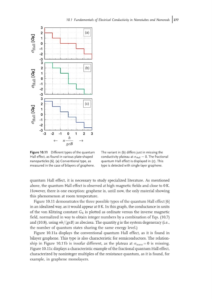
Figure 10.11 demonstrates the three possible types of the quantum Hall effect [6]
in an idealized way, as it would appear at 0 K. In this graph, the conductance in units
of the von Klitzing constant G K is plotted as ordinate versus the inverse magnetic
field, normalized in way to obtain integer numbers by a combination of Eqs. (10.7)
and (10.8), using nh= geB
ð Þas abscissa. The quantity g is the system degeneracy (i.e.,
the number of quantum states sharing the same energy level.)
Figure 10.11a displays the conventional quantum Hall effect, as it is found in
bilayer graphene. This type is also characteristic for semiconductors. The relationship in Figure 10.11b is insofar different, as the plateau at s trans ¼ 0 is missing.
Figure 10.11c displays a characteristic example of the fractional quantum Hall effect,
characterized by noninteger multiples of the resistance quantum, as it is found, for
example, in graphene monolayers.
-3
-2
-1
0
1
2
3
-3
-2
-1
0
1
2
3
σ Hall
[G K
]
-3
-2
-1
0
1
2
3
-3
-2
-1
0
1
2
3
σ Hall
[G K
]
-3 -2 -1
0
1
2
3
-3
-2
-1
0
1
2
3
σ Hall
[G K
]
h
n
geB
←
→
(a)
(b)
(c)
Figure 10.11 Different types of the quantum
Hall effect, as found in various plate-shaped
nanoparticles [6]. (a) Conventional type, as
measured in the case of bilayers of graphene.
The variant in (b) differs just in missing the
conductivity plateau at s Hall ¼ 0. The fractional
quantum Hall effect is displayed in (c). This
type is detected with single-layer graphene.
10.1 Fundamentals of Electrical Conductivity in Nanotubes and Nanorods j277
above, the quantum Hall effect is observed at high magnetic fields and close to 0 K.
However, there is one exception: graphene is, until now, the only material showing
this phenomenon at room temperature.
Figure 10.11 demonstrates the three possible types of the quantum Hall effect [6]
in an idealized way, as it would appear at 0 K. In this graph, the conductance in units
of the von Klitzing constant G K is plotted as ordinate versus the inverse magnetic
field, normalized in way to obtain integer numbers by a combination of Eqs. (10.7)
and (10.8), using nh= geB
ð Þas abscissa. The quantity g is the system degeneracy (i.e.,
the number of quantum states sharing the same energy level.)
Figure 10.11a displays the conventional quantum Hall effect, as it is found in
bilayer graphene. This type is also characteristic for semiconductors. The relationship in Figure 10.11b is insofar different, as the plateau at s trans ¼ 0 is missing.
Figure 10.11c displays a characteristic example of the fractional quantum Hall effect,
characterized by noninteger multiples of the resistance quantum, as it is found, for
example, in graphene monolayers.
-3
-2
-1
0
1
2
3
-3
-2
-1
0
1
2
3
σ Hall
[G K
]
-3
-2
-1
0
1
2
3
-3
-2
-1
0
1
2
3
σ Hall
[G K
]
-3 -2 -1
0
1
2
3
-3
-2
-1
0
1
2
3
σ Hall
[G K
]
h
n
geB
←
→
(a)
(b)
(c)
Figure 10.11 Different types of the quantum
Hall effect, as found in various plate-shaped
nanoparticles [6]. (a) Conventional type, as
measured in the case of bilayers of graphene.
The variant in (b) differs just in missing the
conductivity plateau at s Hall ¼ 0. The fractional
quantum Hall effect is displayed in (c). This
type is detected with single-layer graphene.
10.1 Fundamentals of Electrical Conductivity in Nanotubes and Nanorods j277