

70
Q. Wu et al.
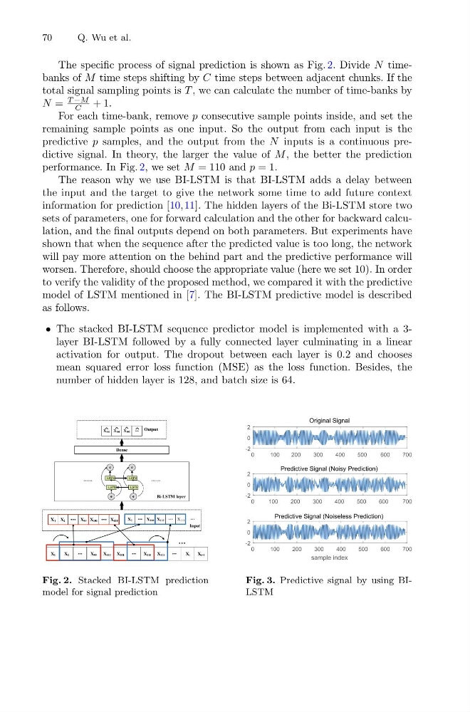
The specific process of signal prediction is shown as Fig. 2. Divide N timebanks of M time steps shifting by C time steps between adjacent chunks. If the
total signal sampling points is T , we can calculate the number of time-banks by
N =
T −M
C
+ 1.
For each time-bank, remove p consecutive sample points inside, and set the
remaining sample points as one input. So the output from each input is the
predictive p samples, and the output from the N inputs is a continuous predictive signal. In theory, the larger the value of M , the better the prediction
performance. In Fig. 2, we set M = 110 and p = 1.
The reason why we use BI-LSTM is that BI-LSTM adds a delay between
the input and the target to give the network some time to add future context
information for prediction [10,11]. The hidden layers of the Bi-LSTM store two
sets of parameters, one for forward calculation and the other for backward calculation, and the final outputs depend on both parameters. But experiments have
shown that when the sequence after the predicted value is too long, the network
will pay more attention on the behind part and the predictive performance will
worsen. Therefore, should choose the appropriate value (here we set 10). In order
to verify the validity of the proposed method, we compared it with the predictive
model of LSTM mentioned in [7]. The BI-LSTM predictive model is described
as follows.
• The stacked BI-LSTM sequence predictor model is implemented with a 3layer BI-LSTM followed by a fully connected layer culminating in a linear
activation for output. The dropout between each layer is 0.2 and chooses
mean squared error loss function (MSE) as the loss function. Besides, the
number of hidden layer is 128, and batch size is 64.
Fig. 2. Stacked BI-LSTM prediction
model for signal prediction
Fig. 3. Predictive signal by using BILSTM
Q. Wu et al.
The specific process of signal prediction is shown as Fig. 2. Divide N timebanks of M time steps shifting by C time steps between adjacent chunks. If the
total signal sampling points is T , we can calculate the number of time-banks by
N =
T −M
C
+ 1.
For each time-bank, remove p consecutive sample points inside, and set the
remaining sample points as one input. So the output from each input is the
predictive p samples, and the output from the N inputs is a continuous predictive signal. In theory, the larger the value of M , the better the prediction
performance. In Fig. 2, we set M = 110 and p = 1.
The reason why we use BI-LSTM is that BI-LSTM adds a delay between
the input and the target to give the network some time to add future context
information for prediction [10,11]. The hidden layers of the Bi-LSTM store two
sets of parameters, one for forward calculation and the other for backward calculation, and the final outputs depend on both parameters. But experiments have
shown that when the sequence after the predicted value is too long, the network
will pay more attention on the behind part and the predictive performance will
worsen. Therefore, should choose the appropriate value (here we set 10). In order
to verify the validity of the proposed method, we compared it with the predictive
model of LSTM mentioned in [7]. The BI-LSTM predictive model is described
as follows.
• The stacked BI-LSTM sequence predictor model is implemented with a 3layer BI-LSTM followed by a fully connected layer culminating in a linear
activation for output. The dropout between each layer is 0.2 and chooses
mean squared error loss function (MSE) as the loss function. Besides, the
number of hidden layer is 128, and batch size is 64.
Fig. 2. Stacked BI-LSTM prediction
model for signal prediction
Fig. 3. Predictive signal by using BILSTM