Feature-Aware Adaptive Denoiser-Selection for Compressed . . .
543
(a) Original Image (b) DnCNN-AMP (c) BMCNN-AMP
(d) BM3D-AMP
(e) Original Image (f) DnCNN-AMP (g) BMCNN-AMP
(h) BM3D-AMP
(i) Original Image
(j) DnCNN-AMP (k) BMCNN-AMP
(l) BM3D-AMP
(m) Original Image (n) DnCNN-AMP (o) BMCNN-AMP
(p) BM3D-AMP
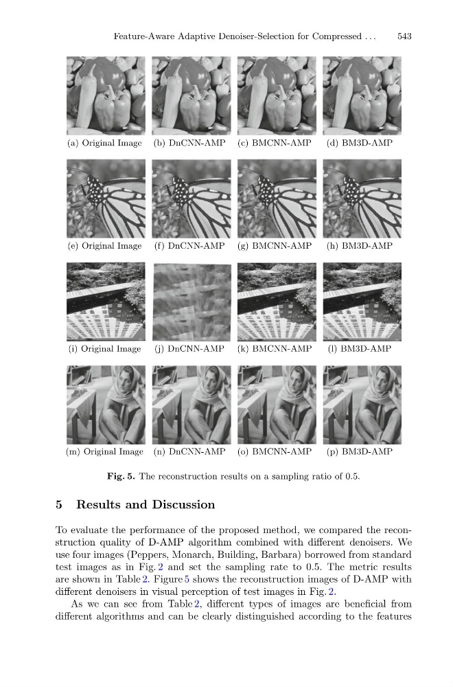
Fig. 5. The reconstruction results on a sampling ratio of 0.5.
5 Results and Discussion
To evaluate the performance of the proposed method, we compared the reconstruction quality of D-AMP algorithm combined with different denoisers. We
use four images (Peppers, Monarch, Building, Barbara) borrowed from standard
test images as in Fig. 2 and set the sampling rate to 0.5. The metric results
are shown in Table 2. Figure 5 shows the reconstruction images of D-AMP with
different denoisers in visual perception of test images in Fig. 2.
As we can see from Table 2, different types of images are beneficial from
different algorithms and can be clearly distinguished according to the features