

L
ðtÞ
¼
1
k
X k
i¼1
y
ðtÞ
i À o
ðtÞ
i
ð3:4Þ
L
ðtÞ
¼
1
k
X k
i¼1
ðy
ðtÞ
i À o
ðtÞ
i Þ
2
ð3:5Þ
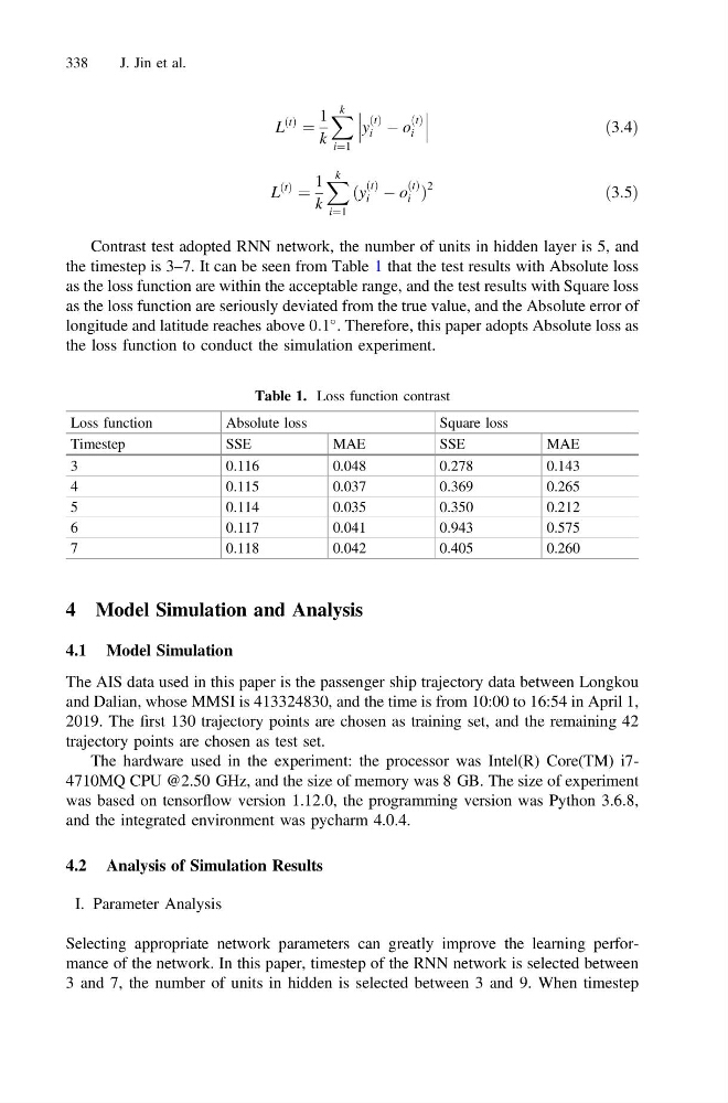
Contrast test adopted RNN network, the number of units in hidden layer is 5, and
the timestep is 3–7. It can be seen from Table 1 that the test results with Absolute loss
as the loss function are within the acceptable range, and the test results with Square loss
as the loss function are seriously deviated from the true value, and the Absolute error of
longitude and latitude reaches above 0:1
. Therefore, this paper adopts Absolute loss as
the loss function to conduct the simulation experiment.
4 Model Simulation and Analysis
4.1 Model Simulation
The AIS data used in this paper is the passenger ship trajectory data between Longkou
and Dalian, whose MMSI is 413324830, and the time is from 10:00 to 16:54 in April 1,
2019. The first 130 trajectory points are chosen as training set, and the remaining 42
trajectory points are chosen as test set.
The hardware used in the experiment: the processor was Intel(R) Core(TM) i74710MQ CPU @2.50 GHz, and the size of memory was 8 GB. The size of experiment
was based on tensorflow version 1.12.0, the programming version was Python 3.6.8,
and the integrated environment was pycharm 4.0.4.
4.2 Analysis of Simulation Results
I. Parameter Analysis
Selecting appropriate network parameters can greatly improve the learning performance of the network. In this paper, timestep of the RNN network is selected between
3 and 7, the number of units in hidden is selected between 3 and 9. When timestep
Table 1. Loss function contrast
Loss function
Absolute loss
Square loss
Timestep
SSE
MAE
SSE
MAE
3
0.116
0.048
0.278
0.143
4
0.115
0.037
0.369
0.265
5
0.114
0.035
0.350
0.212
6
0.117
0.041
0.943
0.575
7
0.118
0.042
0.405
0.260
338
J. Jin et al.
ðtÞ
¼
1
k
X k
i¼1
y
ðtÞ
i À o
ðtÞ
i
ð3:4Þ
L
ðtÞ
¼
1
k
X k
i¼1
ðy
ðtÞ
i À o
ðtÞ
i Þ
2
ð3:5Þ
Contrast test adopted RNN network, the number of units in hidden layer is 5, and
the timestep is 3–7. It can be seen from Table 1 that the test results with Absolute loss
as the loss function are within the acceptable range, and the test results with Square loss
as the loss function are seriously deviated from the true value, and the Absolute error of
longitude and latitude reaches above 0:1
. Therefore, this paper adopts Absolute loss as
the loss function to conduct the simulation experiment.
4 Model Simulation and Analysis
4.1 Model Simulation
The AIS data used in this paper is the passenger ship trajectory data between Longkou
and Dalian, whose MMSI is 413324830, and the time is from 10:00 to 16:54 in April 1,
2019. The first 130 trajectory points are chosen as training set, and the remaining 42
trajectory points are chosen as test set.
The hardware used in the experiment: the processor was Intel(R) Core(TM) i74710MQ CPU @2.50 GHz, and the size of memory was 8 GB. The size of experiment
was based on tensorflow version 1.12.0, the programming version was Python 3.6.8,
and the integrated environment was pycharm 4.0.4.
4.2 Analysis of Simulation Results
I. Parameter Analysis
Selecting appropriate network parameters can greatly improve the learning performance of the network. In this paper, timestep of the RNN network is selected between
3 and 7, the number of units in hidden is selected between 3 and 9. When timestep
Table 1. Loss function contrast
Loss function
Absolute loss
Square loss
Timestep
SSE
MAE
SSE
MAE
3
0.116
0.048
0.278
0.143
4
0.115
0.037
0.369
0.265
5
0.114
0.035
0.350
0.212
6
0.117
0.041
0.943
0.575
7
0.118
0.042
0.405
0.260
338
J. Jin et al.