

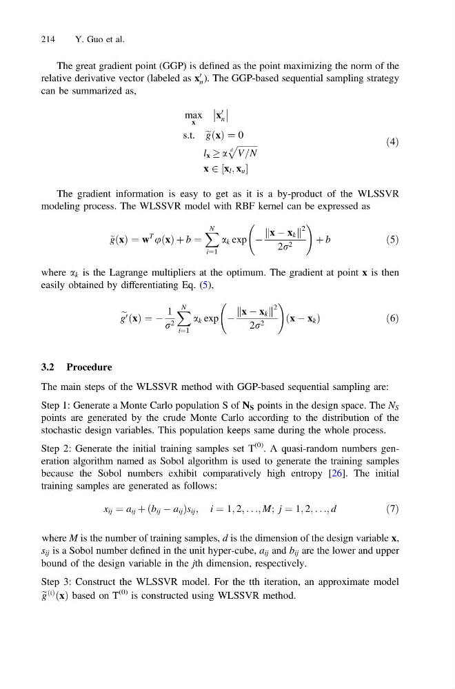
The great gradient point (GGP) is defined as the point maximizing the norm of the
relative derivative vector (labeled as x
0
n ). The GGP-based sequential sampling strategy
can be summarized as,
max
x
x
0
n
s.t. e gðxÞ ¼ 0
l x ! a
ffiffiffiffiffiffiffiffiffi ffi
V=N
d
p
x 2 x l ; x u
½
ð4Þ
The gradient information is easy to get as it is a by-product of the WLSSVR
modeling process. The WLSSVR model with RBF kernel can be expressed as
~ gðxÞ ¼ w
T
uðxÞ þ b ¼
X N
i¼1
a k exp À
x À x k
k
k
2
2r 2
!
þ b
ð5Þ
where a k is the Lagrange multipliers at the optimum. The gradient at point x is then
easily obtained by differentiating Eq. (5),
e
g 0 ðxÞ ¼ À
1
r 2
X N
i¼1
a k exp À
x À x k
k
k
2
2r 2
!
ðx À x k Þ
ð 6Þ
3.2 Procedure
The main steps of the WLSSVR method with GGP-based sequential sampling are:
Step 1: Generate a Monte Carlo population S of N S points in the design space. The N S
points are generated by the crude Monte Carlo according to the distribution of the
stochastic design variables. This population keeps same during the whole process.
Step 2: Generate the initial training samples set T
(0) . A quasi-random numbers generation algorithm named as Sobol algorithm is used to generate the training samples
because the Sobol numbers exhibit comparatively high entropy [26]. The initial
training samples are generated as follows:
x ij ¼ a ij þ ðb ij À a ij Þs ij ; i ¼ 1; 2; . . .; M; j ¼ 1; 2; . . .; d
ð7Þ
where M is the number of training samples, d is the dimension of the design variable x,
s ij is a Sobol number defined in the unit hyper-cube, a ij and b ij are the lower and upper
bound of the design variable in the jth dimension, respectively.
Step 3: Construct the WLSSVR model. For the tth iteration, an approximate model
e g
ðtÞ
ðxÞ based on T
(0) is constructed using WLSSVR method.
214
Y. Guo et al.
relative derivative vector (labeled as x
0
n ). The GGP-based sequential sampling strategy
can be summarized as,
max
x
x
0
n
s.t. e gðxÞ ¼ 0
l x ! a
ffiffiffiffiffiffiffiffiffi ffi
V=N
d
p
x 2 x l ; x u
½
ð4Þ
The gradient information is easy to get as it is a by-product of the WLSSVR
modeling process. The WLSSVR model with RBF kernel can be expressed as
~ gðxÞ ¼ w
T
uðxÞ þ b ¼
X N
i¼1
a k exp À
x À x k
k
k
2
2r 2
!
þ b
ð5Þ
where a k is the Lagrange multipliers at the optimum. The gradient at point x is then
easily obtained by differentiating Eq. (5),
e
g 0 ðxÞ ¼ À
1
r 2
X N
i¼1
a k exp À
x À x k
k
k
2
2r 2
!
ðx À x k Þ
ð 6Þ
3.2 Procedure
The main steps of the WLSSVR method with GGP-based sequential sampling are:
Step 1: Generate a Monte Carlo population S of N S points in the design space. The N S
points are generated by the crude Monte Carlo according to the distribution of the
stochastic design variables. This population keeps same during the whole process.
Step 2: Generate the initial training samples set T
(0) . A quasi-random numbers generation algorithm named as Sobol algorithm is used to generate the training samples
because the Sobol numbers exhibit comparatively high entropy [26]. The initial
training samples are generated as follows:
x ij ¼ a ij þ ðb ij À a ij Þs ij ; i ¼ 1; 2; . . .; M; j ¼ 1; 2; . . .; d
ð7Þ
where M is the number of training samples, d is the dimension of the design variable x,
s ij is a Sobol number defined in the unit hyper-cube, a ij and b ij are the lower and upper
bound of the design variable in the jth dimension, respectively.
Step 3: Construct the WLSSVR model. For the tth iteration, an approximate model
e g
ðtÞ
ðxÞ based on T
(0) is constructed using WLSSVR method.
214
Y. Guo et al.