

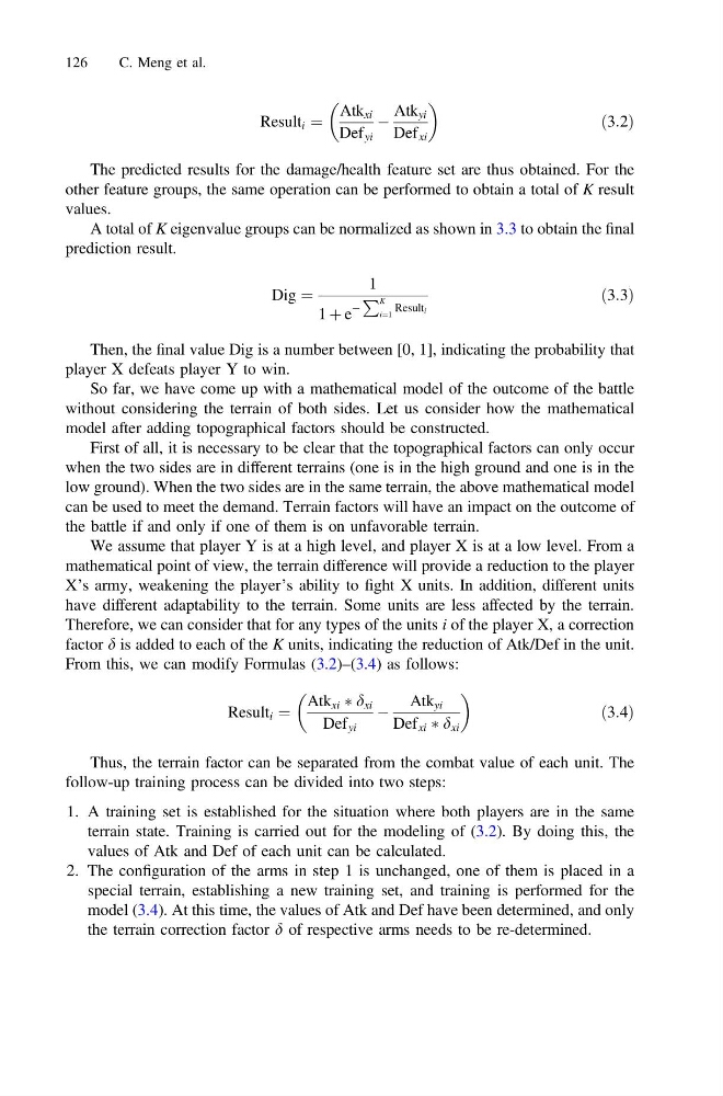
Result i ¼
Atk xi
Def yi
À
Atk yi
Def xi
ð3:2Þ
The predicted results for the damage/health feature set are thus obtained. For the
other feature groups, the same operation can be performed to obtain a total of K result
values.
A total of K eigenvalue groups can be normalized as shown in 3.3 to obtain the final
prediction result.
Dig ¼
1
1 þ e
À
P K
i¼1
Result i
ð3:3Þ
Then, the final value Dig is a number between [0, 1], indicating the probability that
player X defeats player Y to win.
So far, we have come up with a mathematical model of the outcome of the battle
without considering the terrain of both sides. Let us consider how the mathematical
model after adding topographical factors should be constructed.
First of all, it is necessary to be clear that the topographical factors can only occur
when the two sides are in different terrains (one is in the high ground and one is in the
low ground). When the two sides are in the same terrain, the above mathematical model
can be used to meet the demand. Terrain factors will have an impact on the outcome of
the battle if and only if one of them is on unfavorable terrain.
We assume that player Y is at a high level, and player X is at a low level. From a
mathematical point of view, the terrain difference will provide a reduction to the player
X’s army, weakening the player’s ability to fight X units. In addition, different units
have different adaptability to the terrain. Some units are less affected by the terrain.
Therefore, we can consider that for any types of the units i of the player X, a correction
factor d is added to each of the K units, indicating the reduction of Atk/Def in the unit.
From this, we can modify Formulas (3.2)–(3.4) as follows:
Result i ¼
Atk xi à d xi
Def yi
À
Atk yi
Def xi à d xi
ð3:4Þ
Thus, the terrain factor can be separated from the combat value of each unit. The
follow-up training process can be divided into two steps:
1. A training set is established for the situation where both players are in the same
terrain state. Training is carried out for the modeling of (3.2). By doing this, the
values of Atk and Def of each unit can be calculated.
2. The configuration of the arms in step 1 is unchanged, one of them is placed in a
special terrain, establishing a new training set, and training is performed for the
model (3.4). At this time, the values of Atk and Def have been determined, and only
the terrain correction factor d of respective arms needs to be re-determined.
126
C. Meng et al.
Atk xi
Def yi
À
Atk yi
Def xi
ð3:2Þ
The predicted results for the damage/health feature set are thus obtained. For the
other feature groups, the same operation can be performed to obtain a total of K result
values.
A total of K eigenvalue groups can be normalized as shown in 3.3 to obtain the final
prediction result.
Dig ¼
1
1 þ e
À
P K
i¼1
Result i
ð3:3Þ
Then, the final value Dig is a number between [0, 1], indicating the probability that
player X defeats player Y to win.
So far, we have come up with a mathematical model of the outcome of the battle
without considering the terrain of both sides. Let us consider how the mathematical
model after adding topographical factors should be constructed.
First of all, it is necessary to be clear that the topographical factors can only occur
when the two sides are in different terrains (one is in the high ground and one is in the
low ground). When the two sides are in the same terrain, the above mathematical model
can be used to meet the demand. Terrain factors will have an impact on the outcome of
the battle if and only if one of them is on unfavorable terrain.
We assume that player Y is at a high level, and player X is at a low level. From a
mathematical point of view, the terrain difference will provide a reduction to the player
X’s army, weakening the player’s ability to fight X units. In addition, different units
have different adaptability to the terrain. Some units are less affected by the terrain.
Therefore, we can consider that for any types of the units i of the player X, a correction
factor d is added to each of the K units, indicating the reduction of Atk/Def in the unit.
From this, we can modify Formulas (3.2)–(3.4) as follows:
Result i ¼
Atk xi à d xi
Def yi
À
Atk yi
Def xi à d xi
ð3:4Þ
Thus, the terrain factor can be separated from the combat value of each unit. The
follow-up training process can be divided into two steps:
1. A training set is established for the situation where both players are in the same
terrain state. Training is carried out for the modeling of (3.2). By doing this, the
values of Atk and Def of each unit can be calculated.
2. The configuration of the arms in step 1 is unchanged, one of them is placed in a
special terrain, establishing a new training set, and training is performed for the
model (3.4). At this time, the values of Atk and Def have been determined, and only
the terrain correction factor d of respective arms needs to be re-determined.
126
C. Meng et al.