

46
3 Legendre Polynomials and Legendre Functions
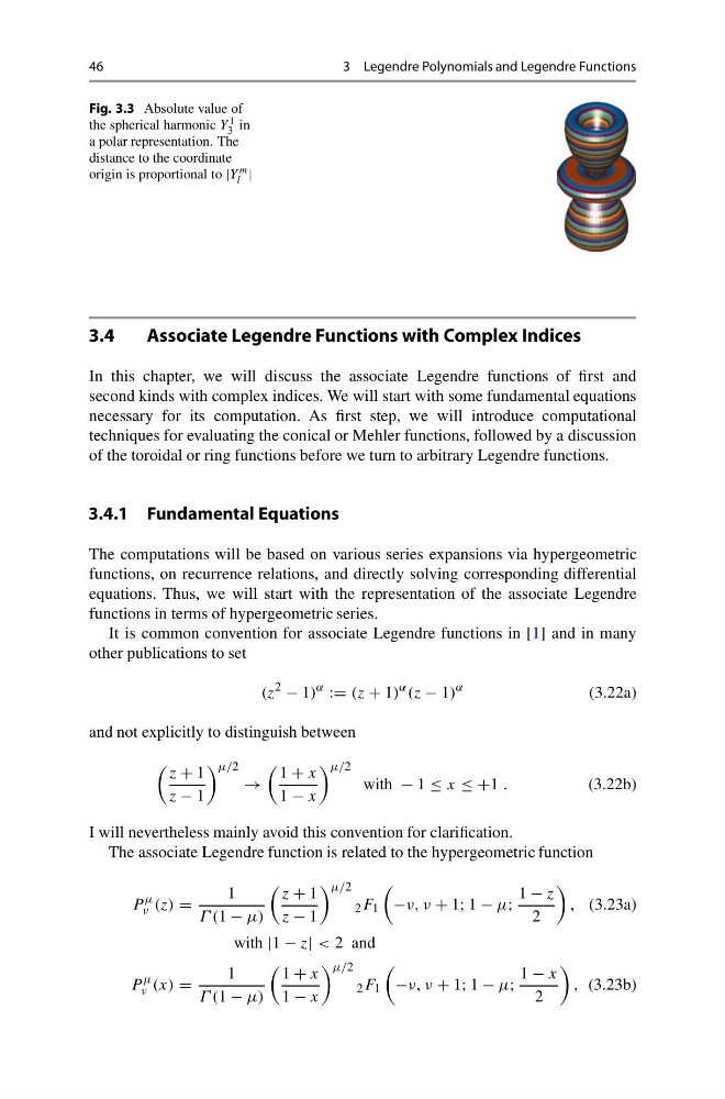
Fig. 3.3 Absolute value of
the spherical harmonic Y 1
3 in
a polar representation. The
distance to the coordinate
origin is proportional to |Y
m
l |
3.4
Associate Legendre Functions with Complex Indices
In this chapter, we will discuss the associate Legendre functions of first and
second kinds with complex indices. We will start with some fundamental equations
necessary for its computation. As first step, we will introduce computational
techniques for evaluating the conical or Mehler functions, followed by a discussion
of the toroidal or ring functions before we turn to arbitrary Legendre functions.
3.4.1 Fundamental Equations
The computations will be based on various series expansions via hypergeometric
functions, on recurrence relations, and directly solving corresponding differential
equations. Thus, we will start with the representation of the associate Legendre
functions in terms of hypergeometric series.
It is common convention for associate Legendre functions in [1] and in many
other publications to set
(z
2
− 1)
α
:= (z + 1)
α (z − 1)
α
(3.22a)
and not explicitly to distinguish between
z + 1
z − 1
μ/2
→
1 + x
1 − x
μ/2
with − 1 ≤ x ≤ +1 .
(3.22b)
I will nevertheless mainly avoid this convention for clarification.
The associate Legendre function is related to the hypergeometric function
P
μ
ν (z) =
1
Γ (1 − μ)
z + 1
z − 1
μ/2
2 F 1
−ν, ν + 1; 1 − μ;
1 − z
2
, (3.23a)
with |1 − z| < 2 and
P
μ
ν (x) =
1
Γ (1 − μ)
1 + x
1 − x
μ/2
2 F 1
−ν, ν + 1; 1 − μ;
1 − x
2
, (3.23b)
3 Legendre Polynomials and Legendre Functions
Fig. 3.3 Absolute value of
the spherical harmonic Y 1
3 in
a polar representation. The
distance to the coordinate
origin is proportional to |Y
m
l |
3.4
Associate Legendre Functions with Complex Indices
In this chapter, we will discuss the associate Legendre functions of first and
second kinds with complex indices. We will start with some fundamental equations
necessary for its computation. As first step, we will introduce computational
techniques for evaluating the conical or Mehler functions, followed by a discussion
of the toroidal or ring functions before we turn to arbitrary Legendre functions.
3.4.1 Fundamental Equations
The computations will be based on various series expansions via hypergeometric
functions, on recurrence relations, and directly solving corresponding differential
equations. Thus, we will start with the representation of the associate Legendre
functions in terms of hypergeometric series.
It is common convention for associate Legendre functions in [1] and in many
other publications to set
(z
2
− 1)
α
:= (z + 1)
α (z − 1)
α
(3.22a)
and not explicitly to distinguish between
z + 1
z − 1
μ/2
→
1 + x
1 − x
μ/2
with − 1 ≤ x ≤ +1 .
(3.22b)
I will nevertheless mainly avoid this convention for clarification.
The associate Legendre function is related to the hypergeometric function
P
μ
ν (z) =
1
Γ (1 − μ)
z + 1
z − 1
μ/2
2 F 1
−ν, ν + 1; 1 − μ;
1 − z
2
, (3.23a)
with |1 − z| < 2 and
P
μ
ν (x) =
1
Γ (1 − μ)
1 + x
1 − x
μ/2
2 F 1
−ν, ν + 1; 1 − μ;
1 − x
2
, (3.23b)