

23.2 Programs and Computational Aspects
273
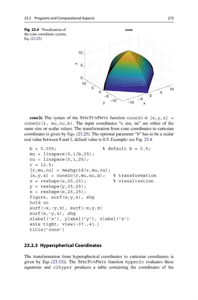
Fig. 23.4 Visualization of
the cone coordinate system,
Eq. (23.25)
cone
10
5
0
z
10
5
0
–5
–10
–10
–5
0
5
10
x
y
cone2c The syntax of the SPECFUNPHYS function cone2c is [x,y,z] =
cone2c(r, mu,nu,b). The input coordinates “r, mu, nu” are either of the
same size or scalar values. The transformation from cone coordinates to cartesian
coordinates is given by Eqs. (23.25). The optional parameter “b” has to be a scalar
real value between 0 and 1, default value is 0.5. Example: see Fig. 23.4
b = 0.005;
% default b = 0.5;
mu = linspace(0,1/b,25);
nu = linspace(0,1,25);
r = 12.5;
[r,mu,nu] = meshgrid(r,mu,nu);
[x,y,z] = cone2c(r,mu,nu,b);
% transformation
z = reshape(z,25,25);
% visualization
y = reshape(y,25,25);
x = reshape(x,25,25);
figure, surf(x,y,z), shg
hold on
surf(-x,-y,z), surf(-x,y,z)
surf(x,-y,z), shg
xlabel(’x’), ylabel(’y’), zlabel(’z’)
axis tight, view(-37.,41.)
title(’cone’)
23.2.3 Hyperspherical Coordinates
The transformation from hyperspherical coordinates to cartesian coordinates is
given by Eqs. (23.33)). The SPECFUNPHYS function hyper2c evaluates these
equations and c2hyper produces a table containing the coordinates of the
273
Fig. 23.4 Visualization of
the cone coordinate system,
Eq. (23.25)
cone
10
5
0
z
10
5
0
–5
–10
–10
–5
0
5
10
x
y
cone2c The syntax of the SPECFUNPHYS function cone2c is [x,y,z] =
cone2c(r, mu,nu,b). The input coordinates “r, mu, nu” are either of the
same size or scalar values. The transformation from cone coordinates to cartesian
coordinates is given by Eqs. (23.25). The optional parameter “b” has to be a scalar
real value between 0 and 1, default value is 0.5. Example: see Fig. 23.4
b = 0.005;
% default b = 0.5;
mu = linspace(0,1/b,25);
nu = linspace(0,1,25);
r = 12.5;
[r,mu,nu] = meshgrid(r,mu,nu);
[x,y,z] = cone2c(r,mu,nu,b);
% transformation
z = reshape(z,25,25);
% visualization
y = reshape(y,25,25);
x = reshape(x,25,25);
figure, surf(x,y,z), shg
hold on
surf(-x,-y,z), surf(-x,y,z)
surf(x,-y,z), shg
xlabel(’x’), ylabel(’y’), zlabel(’z’)
axis tight, view(-37.,41.)
title(’cone’)
23.2.3 Hyperspherical Coordinates
The transformation from hyperspherical coordinates to cartesian coordinates is
given by Eqs. (23.33)). The SPECFUNPHYS function hyper2c evaluates these
equations and c2hyper produces a table containing the coordinates of the