

266
23 Coordinate Systems
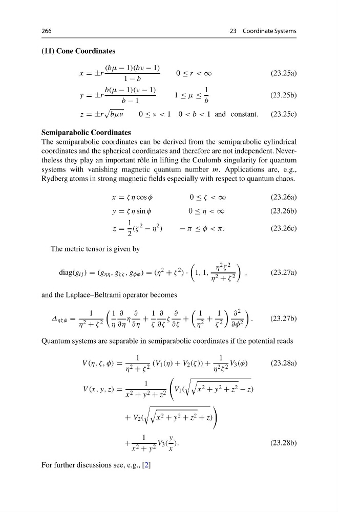
(11) Cone Coordinates
x = ±r
(bμ − 1)(bν − 1)
1 − b
0 ≤ r < ∞
(23.25a)
y = ±r
b(μ − 1)(ν − 1)
b − 1
1 ≤ μ ≤
1
b
(23.25b)
z = ±r
bμν
0 ≤ ν < 1 0 < b < 1 and constant.
(23.25c)
Semiparabolic Coordinates
The semiparabolic coordinates can be derived from the semiparabolic cylindrical
coordinates and the spherical coordinates and therefore are not independent. Nevertheless they play an important rôle in lifting the Coulomb singularity for quantum
systems with vanishing magnetic quantum number m. Applications are, e.g.,
Rydberg atoms in strong magnetic fields especially with respect to quantum chaos.
x = ζ η cos φ
0 ≤ ζ < ∞
(23.26a)
y = ζ η sin φ
0 ≤ η < ∞
(23.26b)
z =
1
2
(ζ
2
− η
2 )
− π ≤ φ < π.
(23.26c)
The metric tensor is given by
diag(g ij ) = (g ηη , g ζ ζ , g φφ ) = (η
2
+ ζ
2 ) ·
1, 1,
η 2 ζ 2
η 2 + ζ 2
,
(23.27a)
and the Laplace–Beltrami operator becomes
Δ ηζ φ =
1
η 2 + ζ 2
1
η
∂
∂η
η
∂
∂η
+
1
ζ
∂
∂ζ
ζ
∂
∂ζ
+
1
η 2 +
1
ζ 2
∂ 2
∂φ 2
.
(23.27b)
Quantum systems are separable in semiparabolic coordinates if the potential reads
V (η, ζ, φ) =
1
η 2 + ζ 2 (V 1 (η) + V 2 (ζ )) +
1
η 2 ζ 2 V 3 (φ)
(23.28a)
V (x, y, z) =
1
x 2 + y 2 + z 2
V 1 (
x 2 + y 2 + z 2 − z)
+ V 2 (
x 2 + y 2 + z 2 + z)
+
1
x 2 + y 2 V 3 (
y
x
).
(23.28b)
For further discussions see, e.g., [2]
23 Coordinate Systems
(11) Cone Coordinates
x = ±r
(bμ − 1)(bν − 1)
1 − b
0 ≤ r < ∞
(23.25a)
y = ±r
b(μ − 1)(ν − 1)
b − 1
1 ≤ μ ≤
1
b
(23.25b)
z = ±r
bμν
0 ≤ ν < 1 0 < b < 1 and constant.
(23.25c)
Semiparabolic Coordinates
The semiparabolic coordinates can be derived from the semiparabolic cylindrical
coordinates and the spherical coordinates and therefore are not independent. Nevertheless they play an important rôle in lifting the Coulomb singularity for quantum
systems with vanishing magnetic quantum number m. Applications are, e.g.,
Rydberg atoms in strong magnetic fields especially with respect to quantum chaos.
x = ζ η cos φ
0 ≤ ζ < ∞
(23.26a)
y = ζ η sin φ
0 ≤ η < ∞
(23.26b)
z =
1
2
(ζ
2
− η
2 )
− π ≤ φ < π.
(23.26c)
The metric tensor is given by
diag(g ij ) = (g ηη , g ζ ζ , g φφ ) = (η
2
+ ζ
2 ) ·
1, 1,
η 2 ζ 2
η 2 + ζ 2
,
(23.27a)
and the Laplace–Beltrami operator becomes
Δ ηζ φ =
1
η 2 + ζ 2
1
η
∂
∂η
η
∂
∂η
+
1
ζ
∂
∂ζ
ζ
∂
∂ζ
+
1
η 2 +
1
ζ 2
∂ 2
∂φ 2
.
(23.27b)
Quantum systems are separable in semiparabolic coordinates if the potential reads
V (η, ζ, φ) =
1
η 2 + ζ 2 (V 1 (η) + V 2 (ζ )) +
1
η 2 ζ 2 V 3 (φ)
(23.28a)
V (x, y, z) =
1
x 2 + y 2 + z 2
V 1 (
x 2 + y 2 + z 2 − z)
+ V 2 (
x 2 + y 2 + z 2 + z)
+
1
x 2 + y 2 V 3 (
y
x
).
(23.28b)
For further discussions see, e.g., [2]