

246
21 Piecewise Interpolation Polynomials
where ψ
(n)
α is the correct value of the wave function at the nodal points and the
summation α runs over all interpolation polynomials. Hence the values, ψ
(n)
α , play
the rôle of the polynomial expansion coefficients on each of the finite elements and
the complete wave function is given by, loosely speaking, putting all pieces together.
21.3.1 Example: The Hydrogen Atom
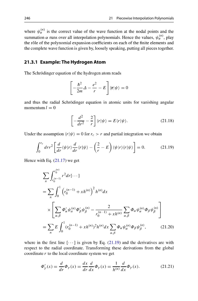
The Schrödinger equation of the hydrogen atom reads
−
¯
h 2
2m
Δ −
e 2
r
− E
= 0
and thus the radial Schrödinger equation in atomic units for vanishing angular
momentum l = 0
−
d 2
dr 2 −
2
r
= E
(21.18)
Under the assumption = 0 for r c > r and partial integration we obtain
r c
0
drr
2
d
dr
d
dr
−
2
r
− E
= 0.
(21.19)
Hence with Eq. (21.17) we get
n
r
(n)
0
r
(n−1)
0
r
2 dr[· · · ]
=
n
1
0
r
(n−1)
0
+ xh
(n)
2
h
(n) dx
×
⎡
⎣
α,β
Φ
α ψ
(n)
α Φ
β ψ
(n)
β −
2
r
(n−1)
0
+ xh (n)
α,β
Φ α ψ
(n)
α Φ β ψ
(n)
β
⎤
⎦
=
n
E
1
0
(r
(n−1)
0
+ xh
(n) )
2 h
(n) dx
α,β
Φ α ψ
(n)
α Φ β ψ
(n)
β ,
(21.20)
where in the first line [· · · ] is given by Eq. (21.19) and the derivatives are with
respect to the radial coordinate. Transforming these derivations from the global
coordinate r to the local coordinate system we get
Φ
γ (x) =
d
dr
Φ γ (x) =
dx
dr
d
dx
Φ γ (x) =
1
h (n)
d
dx
Φ γ (x).
(21.21)
21 Piecewise Interpolation Polynomials
where ψ
(n)
α is the correct value of the wave function at the nodal points and the
summation α runs over all interpolation polynomials. Hence the values, ψ
(n)
α , play
the rôle of the polynomial expansion coefficients on each of the finite elements and
the complete wave function is given by, loosely speaking, putting all pieces together.
21.3.1 Example: The Hydrogen Atom
The Schrödinger equation of the hydrogen atom reads
−
¯
h 2
2m
Δ −
e 2
r
− E
= 0
and thus the radial Schrödinger equation in atomic units for vanishing angular
momentum l = 0
−
d 2
dr 2 −
2
r
= E
(21.18)
Under the assumption = 0 for r c > r and partial integration we obtain
r c
0
drr
2
d
dr
d
dr
−
2
r
− E
= 0.
(21.19)
Hence with Eq. (21.17) we get
n
r
(n)
0
r
(n−1)
0
r
2 dr[· · · ]
=
n
1
0
r
(n−1)
0
+ xh
(n)
2
h
(n) dx
×
⎡
⎣
α,β
Φ
α ψ
(n)
α Φ
β ψ
(n)
β −
2
r
(n−1)
0
+ xh (n)
α,β
Φ α ψ
(n)
α Φ β ψ
(n)
β
⎤
⎦
=
n
E
1
0
(r
(n−1)
0
+ xh
(n) )
2 h
(n) dx
α,β
Φ α ψ
(n)
α Φ β ψ
(n)
β ,
(21.20)
where in the first line [· · · ] is given by Eq. (21.19) and the derivatives are with
respect to the radial coordinate. Transforming these derivations from the global
coordinate r to the local coordinate system we get
Φ
γ (x) =
d
dr
Φ γ (x) =
dx
dr
d
dx
Φ γ (x) =
1
h (n)
d
dx
Φ γ (x).
(21.21)