

242
21 Piecewise Interpolation Polynomials
1
5
7
.
0
5
.
0
5
2
.
0
0
0
0.5
1
Hermite Interpolation polynomial
1
5
7
.
0
5
.
0
5
2
.
0
0
-0.2
0
0.2
1
5
7
.
0
5
.
0
5
2
.
0
0
x
-1
0
1
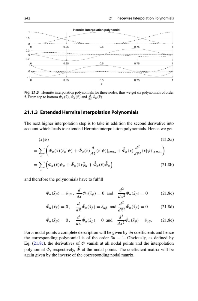
Fig. 21.3 Hermite interpolation polynomials for three nodes, thus we get six polynomials of order
5. From top to bottom Φ α ( ˜
x), ¯
Φ α ( ˜
x) and
d
d ˜
x
¯
Φ α ( ˜
x)
21.1.3 Extended Hermite Interpolation Polynomials
The next higher interpolation step is to take in addition the second derivative into
account which leads to extended Hermite interpolation polynomials. Hence we get
˜
x|ψ
(21.8a)
=
α
Φ α ( ˜
x) ˜
x α |ψ + ¯
Φ α ( ˜
x)
d
d ˜
x
˜
x|ψ x=x α + ¯ ¯
Φ α ( ˜
x)
d 2
d ˜
x 2 ˜
x|ψ x=x α
=
α
Φ α ( ˜
x)ψ α + ¯
Φ α ( ˜
x) ¯
ψ α + ¯ ¯
Φ α ( ˜
x) ¯ ¯
ψ α
(21.8b)
and therefore the polynomials have to fulfill
Φ α ( ˜
x β ) = δ αβ ,
d
d ˜
x
Φ α ( ˜
x β ) = 0 and
d 2
d ˜
x 2 Φ α ( ˜
x β ) = 0
(21.8c)
¯
Φ α ( ˜
x β ) = 0 ,
d
d ˜
x
¯
Φ α ( ˜
x β ) = δ αβ and
d 2
d ˜
x 2
¯
Φ α ( ˜
x β ) = 0
(21.8d)
¯ ¯
Φ α ( ˜
x β ) = 0 ,
d
d ˜
x
¯ ¯
Φ α ( ˜
x β ) = 0 and
d 2
d ˜
x 2
¯ ¯
Φ α ( ˜
x β ) = δ αβ .
(21.8e)
For n nodal points a complete description will be given by 3n coefficients and hence
the corresponding polynomial is of the order 3n − 1. Obviously, as defined by
Eq. (21.8c), the derivatives of Φ vanish at all nodal points and the interpolation
polynomial ¯
Φ, respectively, ¯ ¯
Φ at the nodal points. The coefficient matrix will be
again given by the inverse of the corresponding nodal matrix.
21 Piecewise Interpolation Polynomials
1
5
7
.
0
5
.
0
5
2
.
0
0
0
0.5
1
Hermite Interpolation polynomial
1
5
7
.
0
5
.
0
5
2
.
0
0
-0.2
0
0.2
1
5
7
.
0
5
.
0
5
2
.
0
0
x
-1
0
1
Fig. 21.3 Hermite interpolation polynomials for three nodes, thus we get six polynomials of order
5. From top to bottom Φ α ( ˜
x), ¯
Φ α ( ˜
x) and
d
d ˜
x
¯
Φ α ( ˜
x)
21.1.3 Extended Hermite Interpolation Polynomials
The next higher interpolation step is to take in addition the second derivative into
account which leads to extended Hermite interpolation polynomials. Hence we get
˜
x|ψ
(21.8a)
=
α
Φ α ( ˜
x) ˜
x α |ψ + ¯
Φ α ( ˜
x)
d
d ˜
x
˜
x|ψ x=x α + ¯ ¯
Φ α ( ˜
x)
d 2
d ˜
x 2 ˜
x|ψ x=x α
=
α
Φ α ( ˜
x)ψ α + ¯
Φ α ( ˜
x) ¯
ψ α + ¯ ¯
Φ α ( ˜
x) ¯ ¯
ψ α
(21.8b)
and therefore the polynomials have to fulfill
Φ α ( ˜
x β ) = δ αβ ,
d
d ˜
x
Φ α ( ˜
x β ) = 0 and
d 2
d ˜
x 2 Φ α ( ˜
x β ) = 0
(21.8c)
¯
Φ α ( ˜
x β ) = 0 ,
d
d ˜
x
¯
Φ α ( ˜
x β ) = δ αβ and
d 2
d ˜
x 2
¯
Φ α ( ˜
x β ) = 0
(21.8d)
¯ ¯
Φ α ( ˜
x β ) = 0 ,
d
d ˜
x
¯ ¯
Φ α ( ˜
x β ) = 0 and
d 2
d ˜
x 2
¯ ¯
Φ α ( ˜
x β ) = δ αβ .
(21.8e)
For n nodal points a complete description will be given by 3n coefficients and hence
the corresponding polynomial is of the order 3n − 1. Obviously, as defined by
Eq. (21.8c), the derivatives of Φ vanish at all nodal points and the interpolation
polynomial ¯
Φ, respectively, ¯ ¯
Φ at the nodal points. The coefficient matrix will be
again given by the inverse of the corresponding nodal matrix.