

21.1 Interpolation Polynomials
241
Therefore for n nodal points we obtain 2n linear equations and thus a polynomial of
order 2n − 1.
Example
With ˜
x ∈ [0, +1] and two nodes, ˜
x 0 = 0 and ˜
x 1 = +1, the Hermite interpolation
polynomials will be of order three. For example, for α = 0 we obtain
Φ 0 ( ˜
x) = C 00 + C 01 ˜
x + C 02 ˜
x
2
+ C 03 ˜
x
3
⇒
d
d ˜
x
Φ 0 ( ˜
x) = C 01 + 2C 02 ˜
x + 3C 03 ˜
x
2
¯
Φ 0 ( ˜
x) = ¯
C 00 + ¯
C 01 ˜
x + ¯
C 02 ˜
x
2
+ ¯
C 03 ˜
x
3
⇒
d
d ˜
x
¯
Φ 0 ( ˜
x) = ¯
C 01 + 2 ¯
C 02 ˜
x + 3 ¯
C 03 ˜
x
2 ,
and hence for α = 0 a system of four linear equations at the nodal points:
Φ 0 ( ˜
x 0 ) = C 00 = 1
Φ 0 ( ˜
x 1 ) = C 00 + C 01 + C 02 + C 03 = 0
d
d ˜
x
Φ 0 ( ˜
x 0 ) = C 01 = 0
d
d ˜
x
Φ 0 ( ˜
x 1 ) = C 01 + 2C 02 + 3C 03 = 0
. . .
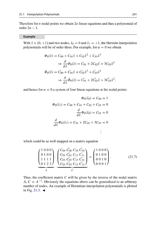
which could be as well mapped on a matrix equation
⎛
⎜
⎜
⎝
1 0 0 0
0 1 0 0
1 1 1 1
0 1 2 3
⎞
⎟
⎟
⎠
A
·
⎛
⎜
⎜
⎝
C 00 ¯
C 00 C 10 ¯
C 10
C 01 ¯
C 01 C 11 ¯
C 11
C 02 ¯
C 02 C 12 ¯
C 12
C 03 ¯
C 03 C 13 ¯
C 13
⎞
⎟
⎟
⎠
C
=
⎛
⎜
⎜
⎝
1 0 0 0
0 1 0 0
0 0 1 0
0 0 0 1
⎞
⎟
⎟
⎠ .
(21.7)
Thus, the coefficient matrix C will be given by the inverse of the nodal matrix
A, C = A −1 . Obviously the equations above can be generalized to an arbitrary
number of nodes. An example of Hermitian interpolation polynomials is plotted
in Fig. 21.3.
241
Therefore for n nodal points we obtain 2n linear equations and thus a polynomial of
order 2n − 1.
Example
With ˜
x ∈ [0, +1] and two nodes, ˜
x 0 = 0 and ˜
x 1 = +1, the Hermite interpolation
polynomials will be of order three. For example, for α = 0 we obtain
Φ 0 ( ˜
x) = C 00 + C 01 ˜
x + C 02 ˜
x
2
+ C 03 ˜
x
3
⇒
d
d ˜
x
Φ 0 ( ˜
x) = C 01 + 2C 02 ˜
x + 3C 03 ˜
x
2
¯
Φ 0 ( ˜
x) = ¯
C 00 + ¯
C 01 ˜
x + ¯
C 02 ˜
x
2
+ ¯
C 03 ˜
x
3
⇒
d
d ˜
x
¯
Φ 0 ( ˜
x) = ¯
C 01 + 2 ¯
C 02 ˜
x + 3 ¯
C 03 ˜
x
2 ,
and hence for α = 0 a system of four linear equations at the nodal points:
Φ 0 ( ˜
x 0 ) = C 00 = 1
Φ 0 ( ˜
x 1 ) = C 00 + C 01 + C 02 + C 03 = 0
d
d ˜
x
Φ 0 ( ˜
x 0 ) = C 01 = 0
d
d ˜
x
Φ 0 ( ˜
x 1 ) = C 01 + 2C 02 + 3C 03 = 0
. . .
which could be as well mapped on a matrix equation
⎛
⎜
⎜
⎝
1 0 0 0
0 1 0 0
1 1 1 1
0 1 2 3
⎞
⎟
⎟
⎠
A
·
⎛
⎜
⎜
⎝
C 00 ¯
C 00 C 10 ¯
C 10
C 01 ¯
C 01 C 11 ¯
C 11
C 02 ¯
C 02 C 12 ¯
C 12
C 03 ¯
C 03 C 13 ¯
C 13
⎞
⎟
⎟
⎠
C
=
⎛
⎜
⎜
⎝
1 0 0 0
0 1 0 0
0 0 1 0
0 0 0 1
⎞
⎟
⎟
⎠ .
(21.7)
Thus, the coefficient matrix C will be given by the inverse of the nodal matrix
A, C = A −1 . Obviously the equations above can be generalized to an arbitrary
number of nodes. An example of Hermitian interpolation polynomials is plotted
in Fig. 21.3.