

21.1 Interpolation Polynomials
239
with correct values at the nodes ˜
x α . For local coordinate values between the nodes,
the wave function will be approximated by the Lagrange interpolation polynomial
Φ α ( ˜
x) =
n
i=0
C αi ˜
x
i .
(21.3)
Example
A Lagrange interpolation polynomial of order n has n + 1 linear independent
coefficients C αi and therefore n + 1 equidistantly distributed nodal points on the
interval 0 ≤ ˜
x ≤ +1. For example, for 3 nodes we get n = 2, ˜
x 0 = 0, ˜
x 1 =
0.5, ˜
x 2 = +1 and therefore a system of three linear equations for fixed index α
Φ 0 ( ˜
x 0 ) = Φ 0 (0) = C 00 = 1
Φ 0 ( ˜
x 1 ) = Φ 0 (0.5) = C 00 +
1
2
C 01 +
1
4
C 02 = 0
Φ 0 ( ˜
x 2 ) = Φ 0 (+1) = C 00 + C 01 + C 02 = 0,
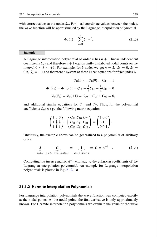
and additional similar equations for Φ 1 and Φ 2 . Thus, for the polynomial
coefficients C αi we get the following matrix equation
⎛
⎝
1 0 0
1
1
2
1
4
1 1 1
⎞
⎠ ·
⎛
⎝
C 00 C 10 C 20
C 01 C 11 C 21
C 02 C 12 C 22
⎞
⎠ =
⎛
⎝
1 0 0
0 1 0
0 0 1
⎞
⎠ .
Obviously, the example above can be generalized to a polynomial of arbitrary
order:
A
nodes
·
C
coeff icient mat rix
=
1
unity mat rix
⇒ C = A
−1 .
(21.4)
Computing the inverse matrix A −1 will lead to the unknown coefficients of the
Lagrangian interpolation polynomial. An example for Lagrange interpolation
polynomials is plotted in Fig. 21.2.
21.1.2 Hermite Interpolation Polynomials
For Lagrange interpolation polynomials the wave function was computed exactly
at the nodal points. At the nodal points the first derivative is only approximately
known. For Hermite interpolation polynomials we evaluate the value of the wave
239
with correct values at the nodes ˜
x α . For local coordinate values between the nodes,
the wave function will be approximated by the Lagrange interpolation polynomial
Φ α ( ˜
x) =
n
i=0
C αi ˜
x
i .
(21.3)
Example
A Lagrange interpolation polynomial of order n has n + 1 linear independent
coefficients C αi and therefore n + 1 equidistantly distributed nodal points on the
interval 0 ≤ ˜
x ≤ +1. For example, for 3 nodes we get n = 2, ˜
x 0 = 0, ˜
x 1 =
0.5, ˜
x 2 = +1 and therefore a system of three linear equations for fixed index α
Φ 0 ( ˜
x 0 ) = Φ 0 (0) = C 00 = 1
Φ 0 ( ˜
x 1 ) = Φ 0 (0.5) = C 00 +
1
2
C 01 +
1
4
C 02 = 0
Φ 0 ( ˜
x 2 ) = Φ 0 (+1) = C 00 + C 01 + C 02 = 0,
and additional similar equations for Φ 1 and Φ 2 . Thus, for the polynomial
coefficients C αi we get the following matrix equation
⎛
⎝
1 0 0
1
1
2
1
4
1 1 1
⎞
⎠ ·
⎛
⎝
C 00 C 10 C 20
C 01 C 11 C 21
C 02 C 12 C 22
⎞
⎠ =
⎛
⎝
1 0 0
0 1 0
0 0 1
⎞
⎠ .
Obviously, the example above can be generalized to a polynomial of arbitrary
order:
A
nodes
·
C
coeff icient mat rix
=
1
unity mat rix
⇒ C = A
−1 .
(21.4)
Computing the inverse matrix A −1 will lead to the unknown coefficients of the
Lagrangian interpolation polynomial. An example for Lagrange interpolation
polynomials is plotted in Fig. 21.2.
21.1.2 Hermite Interpolation Polynomials
For Lagrange interpolation polynomials the wave function was computed exactly
at the nodal points. At the nodal points the first derivative is only approximately
known. For Hermite interpolation polynomials we evaluate the value of the wave