

238
21 Piecewise Interpolation Polynomials
0
2
4
6
8
1 0
1 2
1 4
1 6
1 8
2 0
global coordinates
-0.2
0
0.2
0.4
0.6
0.8
0
0.5
1
local coordinates
0
0.25
0.5
0.75
1
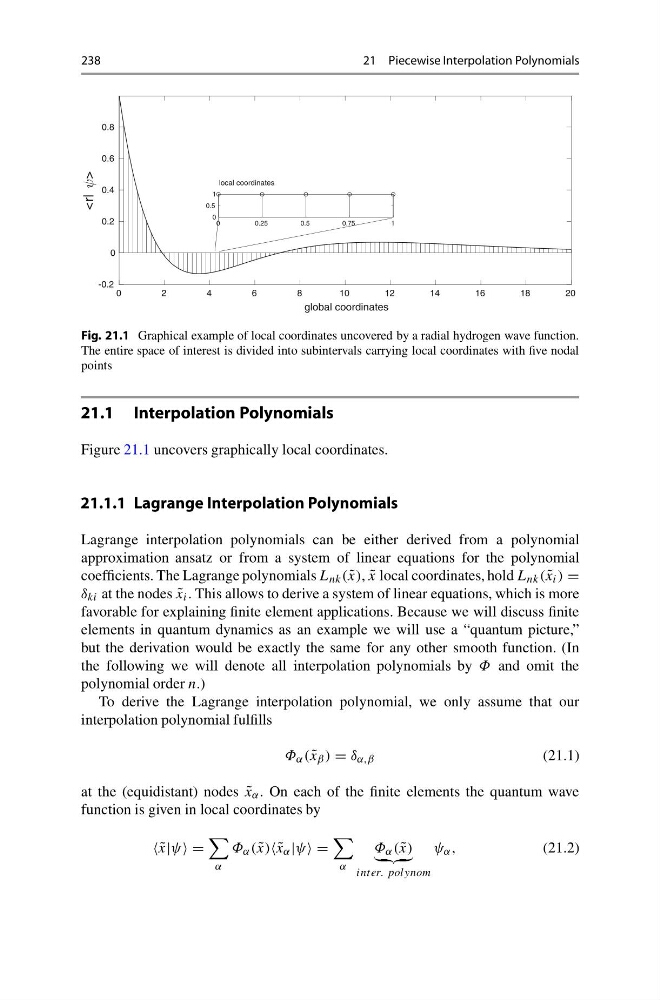
Fig. 21.1 Graphical example of local coordinates uncovered by a radial hydrogen wave function.
The entire space of interest is divided into subintervals carrying local coordinates with five nodal
points
21.1 Interpolation Polynomials
Figure 21.1 uncovers graphically local coordinates.
21.1.1 Lagrange Interpolation Polynomials
Lagrange interpolation polynomials can be either derived from a polynomial
approximation ansatz or from a system of linear equations for the polynomial
coefficients. The Lagrange polynomials L nk ( ˜
x), ˜
x local coordinates, hold L nk ( ˜
x i ) =
δ ki at the nodes ˜
x i . This allows to derive a system of linear equations, which is more
favorable for explaining finite element applications. Because we will discuss finite
elements in quantum dynamics as an example we will use a “quantum picture,”
but the derivation would be exactly the same for any other smooth function. (In
the following we will denote all interpolation polynomials by Φ and omit the
polynomial order n.)
To derive the Lagrange interpolation polynomial, we only assume that our
interpolation polynomial fulfills
Φ α ( ˜
x β ) = δ α,β
(21.1)
at the (equidistant) nodes ˜
x α . On each of the finite elements the quantum wave
function is given in local coordinates by
˜
x|ψ =
α
Φ α ( ˜
x) ˜
x α |ψ =
α
Φ α ( ˜
x)
inter. polynom
ψ α ,
(21.2)
21 Piecewise Interpolation Polynomials
0
2
4
6
8
1 0
1 2
1 4
1 6
1 8
2 0
global coordinates
-0.2
0
0.2
0.4
0.6
0.8
0
0.5
1
local coordinates
0
0.25
0.5
0.75
1
Fig. 21.1 Graphical example of local coordinates uncovered by a radial hydrogen wave function.
The entire space of interest is divided into subintervals carrying local coordinates with five nodal
points
21.1 Interpolation Polynomials
Figure 21.1 uncovers graphically local coordinates.
21.1.1 Lagrange Interpolation Polynomials
Lagrange interpolation polynomials can be either derived from a polynomial
approximation ansatz or from a system of linear equations for the polynomial
coefficients. The Lagrange polynomials L nk ( ˜
x), ˜
x local coordinates, hold L nk ( ˜
x i ) =
δ ki at the nodes ˜
x i . This allows to derive a system of linear equations, which is more
favorable for explaining finite element applications. Because we will discuss finite
elements in quantum dynamics as an example we will use a “quantum picture,”
but the derivation would be exactly the same for any other smooth function. (In
the following we will denote all interpolation polynomials by Φ and omit the
polynomial order n.)
To derive the Lagrange interpolation polynomial, we only assume that our
interpolation polynomial fulfills
Φ α ( ˜
x β ) = δ α,β
(21.1)
at the (equidistant) nodes ˜
x α . On each of the finite elements the quantum wave
function is given in local coordinates by
˜
x|ψ =
α
Φ α ( ˜
x) ˜
x α |ψ =
α
Φ α ( ˜
x)
inter. polynom
ψ α ,
(21.2)