

224
18 Chebyshev Polynomials
0
0.2
0.4
0.6
0.8
1
x
0.6
0.8
1
1.2
1.4
1.6
1.8
y
0
0.5
1
x
0
0.005
0.01
0.015
0.02
0.025
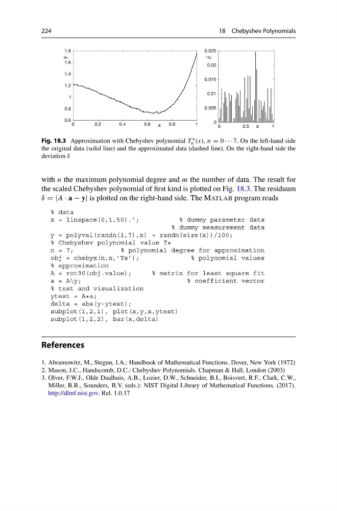
Fig. 18.3 Approximation with Chebyshev polynomial T ∗
n (x), n = 0 · · · 7. On the left-hand side
the original data (solid line) and the approximated data (dashed line). On the right-hand side the
deviation δ
with n the maximum polynomial degree and m the number of data. The result for
the scaled Chebyshev polynomial of first kind is plotted on Fig. 18.3. The residuum
δ = |A · a − y| is plotted on the right-hand side. The MATLAB program reads
% data
x = linspace(0,1,50).’;
% dummy parameter data
% dummy measurement data
y = polyval(randn(1,7),x) + randn(size(x))/100;
% Chebyshev polynomial value T *
n = 7;
% polynomial degree for approximation
obj = chebyx(n,x,’Ts’);
% polynomial values
% approximation
A = rot90(obj.value);
% matrix for least square fit
a = A\y;
% coefficient vector
% test and visualization
ytest = A * a;
delta = abs(y-ytest);
subplot(1,2,1), plot(x,y,x,ytest)
subplot(1,2,2), bar(x,delta)
References
1. Abramowitz, M., Stegun, I.A.: Handbook of Mathematical Functions. Dover, New York (1972)
2. Mason, J.C., Handscomb, D.C.: Chebyshev Polynomials. Chapman & Hall, London (2003)
3. Olver, F.W.J., Olde Daalhuis, A.B., Lozier, D.W., Schneider, B.I., Boisvert, R.F., Clark, C.W.,
Miller, B.R., Sounders, B.V. (eds.): NIST Digital Library of Mathematical Functions. (2017).
http://dlmf.nist.gov. Rel. 1.0.17
18 Chebyshev Polynomials
0
0.2
0.4
0.6
0.8
1
x
0.6
0.8
1
1.2
1.4
1.6
1.8
y
0
0.5
1
x
0
0.005
0.01
0.015
0.02
0.025
Fig. 18.3 Approximation with Chebyshev polynomial T ∗
n (x), n = 0 · · · 7. On the left-hand side
the original data (solid line) and the approximated data (dashed line). On the right-hand side the
deviation δ
with n the maximum polynomial degree and m the number of data. The result for
the scaled Chebyshev polynomial of first kind is plotted on Fig. 18.3. The residuum
δ = |A · a − y| is plotted on the right-hand side. The MATLAB program reads
% data
x = linspace(0,1,50).’;
% dummy parameter data
% dummy measurement data
y = polyval(randn(1,7),x) + randn(size(x))/100;
% Chebyshev polynomial value T *
n = 7;
% polynomial degree for approximation
obj = chebyx(n,x,’Ts’);
% polynomial values
% approximation
A = rot90(obj.value);
% matrix for least square fit
a = A\y;
% coefficient vector
% test and visualization
ytest = A * a;
delta = abs(y-ytest);
subplot(1,2,1), plot(x,y,x,ytest)
subplot(1,2,2), bar(x,delta)
References
1. Abramowitz, M., Stegun, I.A.: Handbook of Mathematical Functions. Dover, New York (1972)
2. Mason, J.C., Handscomb, D.C.: Chebyshev Polynomials. Chapman & Hall, London (2003)
3. Olver, F.W.J., Olde Daalhuis, A.B., Lozier, D.W., Schneider, B.I., Boisvert, R.F., Clark, C.W.,
Miller, B.R., Sounders, B.V. (eds.): NIST Digital Library of Mathematical Functions. (2017).
http://dlmf.nist.gov. Rel. 1.0.17