

18.2 Computational Aspects and Programs
223
-0.5
0
0.5
1
1.5
x
-2
0
2
4
6
8
10
fun
T
T-s
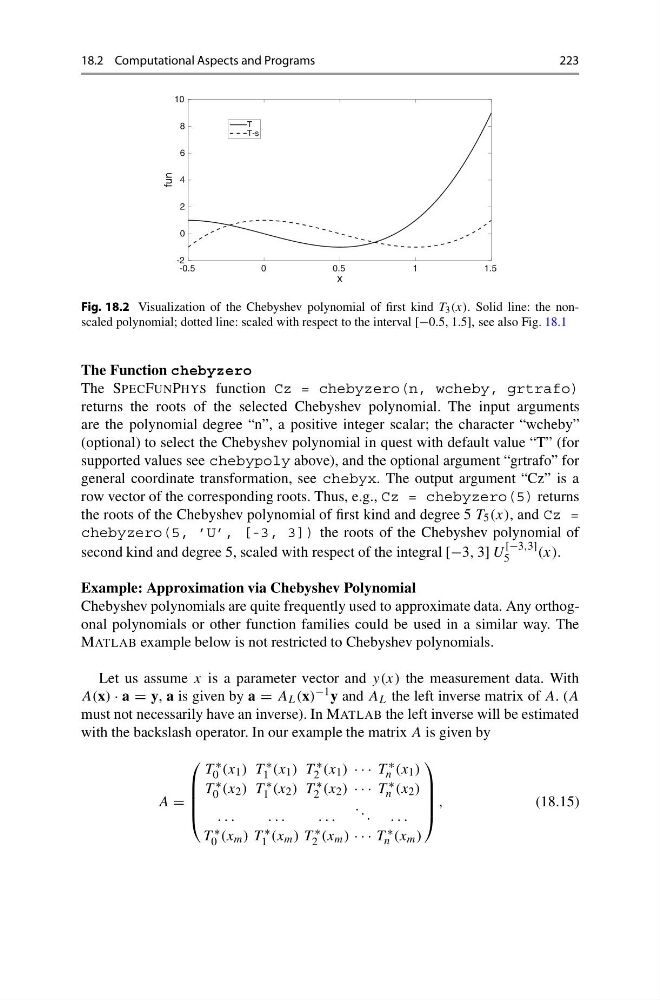
Fig. 18.2 Visualization of the Chebyshev polynomial of first kind T 3 (x). Solid line: the nonscaled polynomial; dotted line: scaled with respect to the interval [−0.5, 1.5], see also Fig. 18.1
The Function chebyzero
The SPECFUNPHYS function Cz = chebyzero(n, wcheby, grtrafo)
returns the roots of the selected Chebyshev polynomial. The input arguments
are the polynomial degree “n”, a positive integer scalar; the character “wcheby”
(optional) to select the Chebyshev polynomial in quest with default value “T” (for
supported values see chebypoly above), and the optional argument “grtrafo” for
general coordinate transformation, see chebyx. The output argument “Cz” is a
row vector of the corresponding roots. Thus, e.g., Cz = chebyzero(5) returns
the roots of the Chebyshev polynomial of first kind and degree 5 T 5 (x), and Cz =
chebyzero(5, ’U’, [-3, 3]) the roots of the Chebyshev polynomial of
second kind and degree 5, scaled with respect of the integral [−3, 3] U
[−3,3]
5
(x).
Example: Approximation via Chebyshev Polynomial
Chebyshev polynomials are quite frequently used to approximate data. Any orthogonal polynomials or other function families could be used in a similar way. The
MATLAB example below is not restricted to Chebyshev polynomials.
Let us assume x is a parameter vector and y(x) the measurement data. With
A(x) · a = y, a is given by a = A L (x) −1 y and A L the left inverse matrix of A. (A
must not necessarily have an inverse). In MATLAB the left inverse will be estimated
with the backslash operator. In our example the matrix A is given by
A =
⎛
⎜
⎜
⎜
⎝
T ∗
0 (x 1 ) T ∗
1 (x 1 ) T ∗
2 (x 1 ) · · · T ∗
n (x 1 )
T ∗
0 (x 2 ) T ∗
1 (x 2 ) T ∗
2 (x 2 ) · · · T ∗
n (x 2 )
. . .
. . .
. . .
. . . . . .
T ∗
0 (x m ) T ∗
1 (x m ) T ∗
2 (x m ) · · · T ∗
n (x m )
⎞
⎟
⎟
⎟
⎠
,
(18.15)
223
-0.5
0
0.5
1
1.5
x
-2
0
2
4
6
8
10
fun
T
T-s
Fig. 18.2 Visualization of the Chebyshev polynomial of first kind T 3 (x). Solid line: the nonscaled polynomial; dotted line: scaled with respect to the interval [−0.5, 1.5], see also Fig. 18.1
The Function chebyzero
The SPECFUNPHYS function Cz = chebyzero(n, wcheby, grtrafo)
returns the roots of the selected Chebyshev polynomial. The input arguments
are the polynomial degree “n”, a positive integer scalar; the character “wcheby”
(optional) to select the Chebyshev polynomial in quest with default value “T” (for
supported values see chebypoly above), and the optional argument “grtrafo” for
general coordinate transformation, see chebyx. The output argument “Cz” is a
row vector of the corresponding roots. Thus, e.g., Cz = chebyzero(5) returns
the roots of the Chebyshev polynomial of first kind and degree 5 T 5 (x), and Cz =
chebyzero(5, ’U’, [-3, 3]) the roots of the Chebyshev polynomial of
second kind and degree 5, scaled with respect of the integral [−3, 3] U
[−3,3]
5
(x).
Example: Approximation via Chebyshev Polynomial
Chebyshev polynomials are quite frequently used to approximate data. Any orthogonal polynomials or other function families could be used in a similar way. The
MATLAB example below is not restricted to Chebyshev polynomials.
Let us assume x is a parameter vector and y(x) the measurement data. With
A(x) · a = y, a is given by a = A L (x) −1 y and A L the left inverse matrix of A. (A
must not necessarily have an inverse). In MATLAB the left inverse will be estimated
with the backslash operator. In our example the matrix A is given by
A =
⎛
⎜
⎜
⎜
⎝
T ∗
0 (x 1 ) T ∗
1 (x 1 ) T ∗
2 (x 1 ) · · · T ∗
n (x 1 )
T ∗
0 (x 2 ) T ∗
1 (x 2 ) T ∗
2 (x 2 ) · · · T ∗
n (x 2 )
. . .
. . .
. . .
. . . . . .
T ∗
0 (x m ) T ∗
1 (x m ) T ∗
2 (x m ) · · · T ∗
n (x m )
⎞
⎟
⎟
⎟
⎠
,
(18.15)