

188
15 Orthogonal Polynomials: General Aspects
>> info
info =
4x1 cell array
{’Gegenbauer Polynomial’
}
{’lambda = 3.1416’
}
{’Integration with weight function’}
{’Integration interval: -1 1’
}
The output variables are: “Cpint” the indefinite Integral of the polynomial
product, if it exists. “prodtab” a table of the polynomial orders of the product
polynomials, “Cpintvalue” the definite integral values, “info” some general
information, and “Cprod” the table of the product of the polynomials before
integration. This value could be useful in case of a weight function, because then
“Cpint” will be empty.
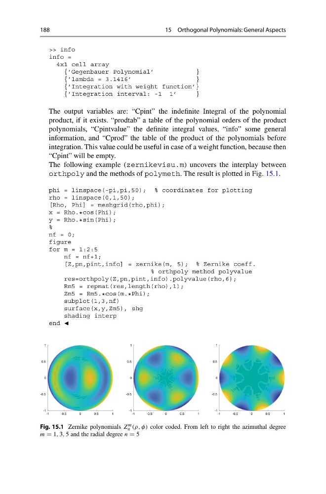
The following example (zernikevisu.m) uncovers the interplay between
orthpoly and the methods of polymeth. The result is plotted in Fig. 15.1.
phi = linspace(-pi,pi,50); % coordinates for plotting
rho = linspace(0,1,50);
[Rho, Phi] = meshgrid(rho,phi);
x = Rho. * cos(Phi);
y = Rho. * sin(Phi);
%
nf = 0;
figure
for m = 1:2:5
nf = nf+1;
[Z,pn,pint,info] = zernike(m, 5); % Zernike coeff.
% orthpoly method polyvalue
res=orthpoly(Z,pn,pint,info).polyvalue(rho,6);
Rm5 = repmat(res,length(rho),1);
Zm5 = Rm5. * cos(m. * Phi);
subplot(1,3,nf)
surface(x,y,Zm5), shg
shading interp
end
-1
-0.5
0
0.5
1
-1
-0.5
0
0.5
1
-1
-0.5
0
0.5
1
-1
-0.5
0
0.5
1
-1
-0.5
0
0.5
1
-1
-0.5
0
0.5
1
Fig. 15.1 Zernike polynomials Z m
n (ρ, φ) color coded. From left to right the azimuthal degree
m = 1, 3, 5 and the radial degree n = 5
15 Orthogonal Polynomials: General Aspects
>> info
info =
4x1 cell array
{’Gegenbauer Polynomial’
}
{’lambda = 3.1416’
}
{’Integration with weight function’}
{’Integration interval: -1 1’
}
The output variables are: “Cpint” the indefinite Integral of the polynomial
product, if it exists. “prodtab” a table of the polynomial orders of the product
polynomials, “Cpintvalue” the definite integral values, “info” some general
information, and “Cprod” the table of the product of the polynomials before
integration. This value could be useful in case of a weight function, because then
“Cpint” will be empty.
The following example (zernikevisu.m) uncovers the interplay between
orthpoly and the methods of polymeth. The result is plotted in Fig. 15.1.
phi = linspace(-pi,pi,50); % coordinates for plotting
rho = linspace(0,1,50);
[Rho, Phi] = meshgrid(rho,phi);
x = Rho. * cos(Phi);
y = Rho. * sin(Phi);
%
nf = 0;
figure
for m = 1:2:5
nf = nf+1;
[Z,pn,pint,info] = zernike(m, 5); % Zernike coeff.
% orthpoly method polyvalue
res=orthpoly(Z,pn,pint,info).polyvalue(rho,6);
Rm5 = repmat(res,length(rho),1);
Zm5 = Rm5. * cos(m. * Phi);
subplot(1,3,nf)
surface(x,y,Zm5), shg
shading interp
end
-1
-0.5
0
0.5
1
-1
-0.5
0
0.5
1
-1
-0.5
0
0.5
1
-1
-0.5
0
0.5
1
-1
-0.5
0
0.5
1
-1
-0.5
0
0.5
1
Fig. 15.1 Zernike polynomials Z m
n (ρ, φ) color coded. From left to right the azimuthal degree
m = 1, 3, 5 and the radial degree n = 5