

References
179
z
-4
-3
-2
-1
0
1
2
3
4
real
-0.4
-0.3
-0.2
-0.1
0
0.1
0.2
imag
0
0.5
1
1.5
2
2.5
3
0
0.5
1
1.5
2
z
0
50
100
150
real
0
200
400
600
800
1000
1200
1400
1600
1800
imag
0
0 . 5
1
1 . 5
2
z
-4
-2
0
2
4
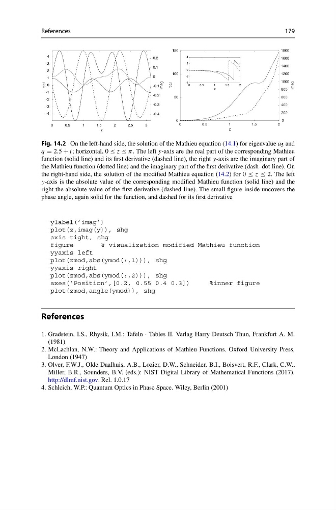
Fig. 14.2 On the left-hand side, the solution of the Mathieu equation (14.1) for eigenvalue a 5 and
q = 2.5 + i; horizontal, 0 ≤ z ≤ π. The left y-axis are the real part of the corresponding Mathieu
function (solid line) and its first derivative (dashed line), the right y-axis are the imaginary part of
the Mathieu function (dotted line) and the imaginary part of the first derivative (dash–dot line). On
the right-hand side, the solution of the modified Mathieu equation (14.2) for 0 ≤ z ≤ 2. The left
y-axis is the absolute value of the corresponding modified Mathieu function (solid line) and the
right the absolute value of the first derivative (dashed line). The small figure inside uncovers the
phase angle, again solid for the function, and dashed for its first derivative
ylabel(’imag’)
plot(z,imag(y)), shg
axis tight, shg
figure
% visualization modified Mathieu function
yyaxis left
plot(zmod,abs(ymod(:,1))), shg
yyaxis right
plot(zmod,abs(ymod(:,2))), shg
axes(’Position’,[0.2, 0.55 0.4 0.3])
%inner figure
plot(zmod,angle(ymod)), shg
References
1. Gradstein, I.S., Rhysik, I.M.: Tafeln · Tables II. Verlag Harry Deutsch Thun, Frankfurt A. M.
(1981)
2. McLachlan, N.W.: Theory and Applications of Mathieu Functions. Oxford University Press,
London (1947)
3. Olver, F.W.J., Olde Daalhuis, A.B., Lozier, D.W., Schneider, B.I., Boisvert, R.F., Clark, C.W.,
Miller, B.R., Sounders, B.V. (eds.): NIST Digital Library of Mathematical Functions (2017).
http://dlmf.nist.gov. Rel. 1.0.17
4. Schleich, W.P.: Quantum Optics in Phase Space. Wiley, Berlin (2001)
179
z
-4
-3
-2
-1
0
1
2
3
4
real
-0.4
-0.3
-0.2
-0.1
0
0.1
0.2
imag
0
0.5
1
1.5
2
2.5
3
0
0.5
1
1.5
2
z
0
50
100
150
real
0
200
400
600
800
1000
1200
1400
1600
1800
imag
0
0 . 5
1
1 . 5
2
z
-4
-2
0
2
4
Fig. 14.2 On the left-hand side, the solution of the Mathieu equation (14.1) for eigenvalue a 5 and
q = 2.5 + i; horizontal, 0 ≤ z ≤ π. The left y-axis are the real part of the corresponding Mathieu
function (solid line) and its first derivative (dashed line), the right y-axis are the imaginary part of
the Mathieu function (dotted line) and the imaginary part of the first derivative (dash–dot line). On
the right-hand side, the solution of the modified Mathieu equation (14.2) for 0 ≤ z ≤ 2. The left
y-axis is the absolute value of the corresponding modified Mathieu function (solid line) and the
right the absolute value of the first derivative (dashed line). The small figure inside uncovers the
phase angle, again solid for the function, and dashed for its first derivative
ylabel(’imag’)
plot(z,imag(y)), shg
axis tight, shg
figure
% visualization modified Mathieu function
yyaxis left
plot(zmod,abs(ymod(:,1))), shg
yyaxis right
plot(zmod,abs(ymod(:,2))), shg
axes(’Position’,[0.2, 0.55 0.4 0.3])
%inner figure
plot(zmod,angle(ymod)), shg
References
1. Gradstein, I.S., Rhysik, I.M.: Tafeln · Tables II. Verlag Harry Deutsch Thun, Frankfurt A. M.
(1981)
2. McLachlan, N.W.: Theory and Applications of Mathieu Functions. Oxford University Press,
London (1947)
3. Olver, F.W.J., Olde Daalhuis, A.B., Lozier, D.W., Schneider, B.I., Boisvert, R.F., Clark, C.W.,
Miller, B.R., Sounders, B.V. (eds.): NIST Digital Library of Mathematical Functions (2017).
http://dlmf.nist.gov. Rel. 1.0.17
4. Schleich, W.P.: Quantum Optics in Phase Space. Wiley, Berlin (2001)