

178
14 Mathieu Functions
0
2
4
6
8
1 0
q
-15
-10
-5
0
5
10
15
20
25
a(0)
a(1)
a(2)
a(3)
a(4)
b(1)
b(2)
b(3)
b(4)
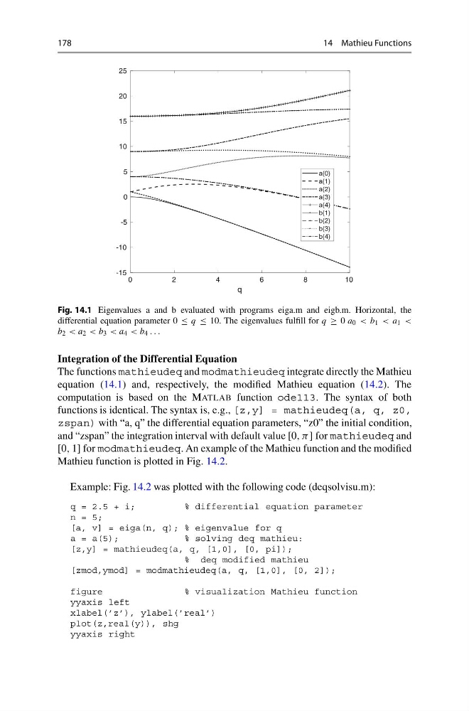
Fig. 14.1 Eigenvalues a and b evaluated with programs eiga.m and eigb.m. Horizontal, the
differential equation parameter 0 ≤ q ≤ 10. The eigenvalues fulfill for q ≥ 0 a 0 < b 1 < a 1 <
b 2 < a 2 < b 3 < a 4 < b 4 . . .
Integration of the Differential Equation
The functions mathieudeq and modmathieudeq integrate directly the Mathieu
equation (14.1) and, respectively, the modified Mathieu equation (14.2). The
computation is based on the MATLAB function ode113. The syntax of both
functions is identical. The syntax is, e.g., [z,y] = mathieudeq(a, q, z0,
zspan) with “a, q” the differential equation parameters, “z0” the initial condition,
and “zspan” the integration interval with default value [0, π] for mathieudeq and
[0, 1] for modmathieudeq. An example of the Mathieu function and the modified
Mathieu function is plotted in Fig. 14.2.
Example: Fig. 14.2 was plotted with the following code (deqsolvisu.m):
q = 2.5 + i;
% differential equation parameter
n = 5;
[a, v] = eiga(n, q); % eigenvalue for q
a = a(5);
% solving deq mathieu:
[z,y] = mathieudeq(a, q, [1,0], [0, pi]);
% deq modified mathieu
[zmod,ymod] = modmathieudeq(a, q, [1,0], [0, 2]);
figure
% visualization Mathieu function
yyaxis left
xlabel(’z’), ylabel(’real’)
plot(z,real(y)), shg
yyaxis right
14 Mathieu Functions
0
2
4
6
8
1 0
q
-15
-10
-5
0
5
10
15
20
25
a(0)
a(1)
a(2)
a(3)
a(4)
b(1)
b(2)
b(3)
b(4)
Fig. 14.1 Eigenvalues a and b evaluated with programs eiga.m and eigb.m. Horizontal, the
differential equation parameter 0 ≤ q ≤ 10. The eigenvalues fulfill for q ≥ 0 a 0 < b 1 < a 1 <
b 2 < a 2 < b 3 < a 4 < b 4 . . .
Integration of the Differential Equation
The functions mathieudeq and modmathieudeq integrate directly the Mathieu
equation (14.1) and, respectively, the modified Mathieu equation (14.2). The
computation is based on the MATLAB function ode113. The syntax of both
functions is identical. The syntax is, e.g., [z,y] = mathieudeq(a, q, z0,
zspan) with “a, q” the differential equation parameters, “z0” the initial condition,
and “zspan” the integration interval with default value [0, π] for mathieudeq and
[0, 1] for modmathieudeq. An example of the Mathieu function and the modified
Mathieu function is plotted in Fig. 14.2.
Example: Fig. 14.2 was plotted with the following code (deqsolvisu.m):
q = 2.5 + i;
% differential equation parameter
n = 5;
[a, v] = eiga(n, q); % eigenvalue for q
a = a(5);
% solving deq mathieu:
[z,y] = mathieudeq(a, q, [1,0], [0, pi]);
% deq modified mathieu
[zmod,ymod] = modmathieudeq(a, q, [1,0], [0, 2]);
figure
% visualization Mathieu function
yyaxis left
xlabel(’z’), ylabel(’real’)
plot(z,real(y)), shg
yyaxis right