

14.2 Fundamental Equations and Computation
173
F e n (z, q) = −i f e n (i z, q) n ∈ N
(14.28d)
Ge n (z, q) = ge n (i z, q) n ∈ N
∗ .
(14.28e)
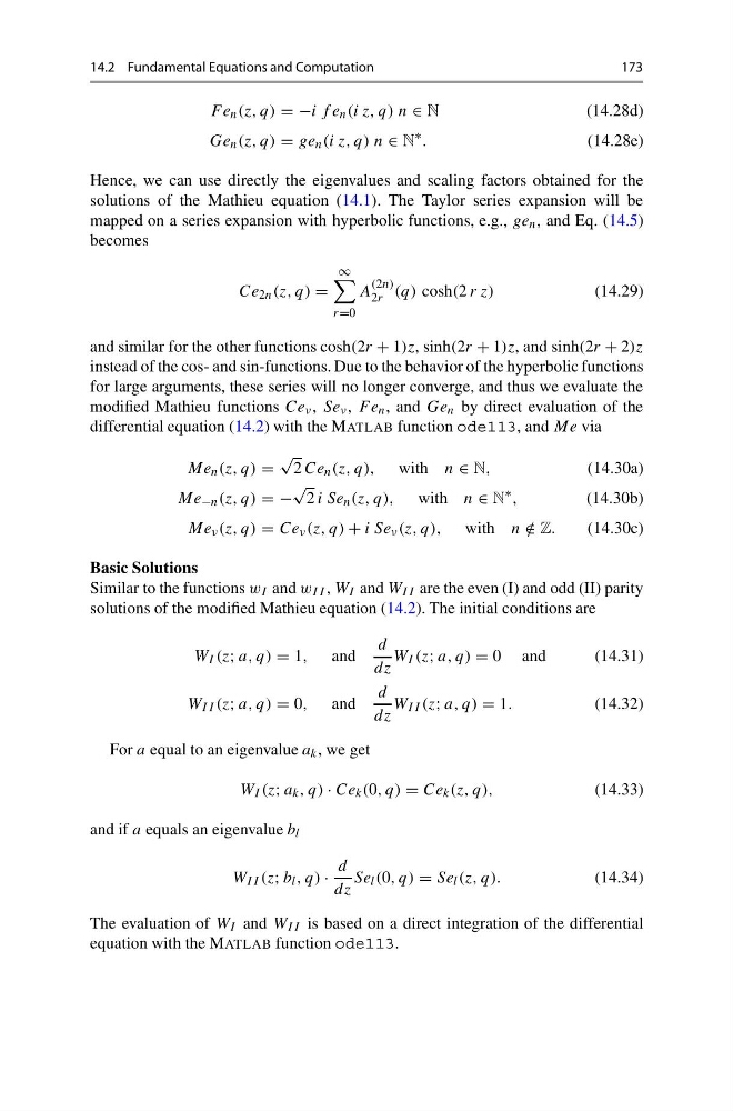
Hence, we can use directly the eigenvalues and scaling factors obtained for the
solutions of the Mathieu equation (14.1). The Taylor series expansion will be
mapped on a series expansion with hyperbolic functions, e.g., ge n , and Eq. (14.5)
becomes
Ce 2n (z, q) =
∞
r=0
A
(2n)
2r (q) cosh(2 r z)
(14.29)
and similar for the other functions cosh(2r + 1)z, sinh(2r + 1)z, and sinh(2r + 2)z
instead of the cos- and sin-functions. Due to the behavior of the hyperbolic functions
for large arguments, these series will no longer converge, and thus we evaluate the
modified Mathieu functions Ce ν , Se ν , F e n , and Ge n by direct evaluation of the
differential equation (14.2) with the MATLAB function ode113, and Me via
Me n (z, q) =
√
2 Ce n (z, q), with n ∈ N,
(14.30a)
Me −n (z, q) = −
√
2 i Se n (z, q), with n ∈ N
∗ ,
(14.30b)
Me ν (z, q) = Ce ν (z, q) + i Se ν (z, q), with n /
∈ Z.
(14.30c)
Basic Solutions
Similar to the functions w I and w I I , W I and W I I are the even (I) and odd (II) parity
solutions of the modified Mathieu equation (14.2). The initial conditions are
W I (z; a, q) = 1, and
d
dz
W I (z; a, q) = 0 and
(14.31)
W I I (z; a, q) = 0, and
d
dz
W I I (z; a, q) = 1.
(14.32)
For a equal to an eigenvalue a k , we get
W I (z; a k , q) · Ce k (0, q) = Ce k (z, q),
(14.33)
and if a equals an eigenvalue b l
W I I (z; b l , q) ·
d
dz
Se l (0, q) = Se l (z, q).
(14.34)
The evaluation of W I and W I I is based on a direct integration of the differential
equation with the MATLAB function ode113.
173
F e n (z, q) = −i f e n (i z, q) n ∈ N
(14.28d)
Ge n (z, q) = ge n (i z, q) n ∈ N
∗ .
(14.28e)
Hence, we can use directly the eigenvalues and scaling factors obtained for the
solutions of the Mathieu equation (14.1). The Taylor series expansion will be
mapped on a series expansion with hyperbolic functions, e.g., ge n , and Eq. (14.5)
becomes
Ce 2n (z, q) =
∞
r=0
A
(2n)
2r (q) cosh(2 r z)
(14.29)
and similar for the other functions cosh(2r + 1)z, sinh(2r + 1)z, and sinh(2r + 2)z
instead of the cos- and sin-functions. Due to the behavior of the hyperbolic functions
for large arguments, these series will no longer converge, and thus we evaluate the
modified Mathieu functions Ce ν , Se ν , F e n , and Ge n by direct evaluation of the
differential equation (14.2) with the MATLAB function ode113, and Me via
Me n (z, q) =
√
2 Ce n (z, q), with n ∈ N,
(14.30a)
Me −n (z, q) = −
√
2 i Se n (z, q), with n ∈ N
∗ ,
(14.30b)
Me ν (z, q) = Ce ν (z, q) + i Se ν (z, q), with n /
∈ Z.
(14.30c)
Basic Solutions
Similar to the functions w I and w I I , W I and W I I are the even (I) and odd (II) parity
solutions of the modified Mathieu equation (14.2). The initial conditions are
W I (z; a, q) = 1, and
d
dz
W I (z; a, q) = 0 and
(14.31)
W I I (z; a, q) = 0, and
d
dz
W I I (z; a, q) = 1.
(14.32)
For a equal to an eigenvalue a k , we get
W I (z; a k , q) · Ce k (0, q) = Ce k (z, q),
(14.33)
and if a equals an eigenvalue b l
W I I (z; b l , q) ·
d
dz
Se l (0, q) = Se l (z, q).
(14.34)
The evaluation of W I and W I I is based on a direct integration of the differential
equation with the MATLAB function ode113.