

172
14 Mathieu Functions
with the normalization condition
∞
r=−∞
c
(ν)
2r (q)
2 = 1.
(14.25e)
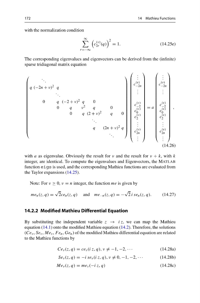
The corresponding eigenvalues and eigenvectors can be derived from the (infinite)
sparse tridiagonal matrix equation
⎛
⎜
⎜
⎜
⎜
⎜
⎜
⎜
⎜
⎜
⎜
⎜
⎜
⎜
⎜
⎜
⎜
⎜
⎜
⎝
. . .
q (−2n + ν) 2 q
. . .
0
q (−2 + ν) 2 q
0
0
q
ν 2
q
0
0
q (2 + ν) 2
q
0
. . .
q
(2n + ν) 2 q
. . .
⎞
⎟
⎟
⎟
⎟
⎟
⎟
⎟
⎟
⎟
⎟
⎟
⎟
⎟
⎟
⎟
⎟
⎟
⎟
⎠
⎛
⎜
⎜
⎜
⎜
⎜
⎜
⎜
⎜
⎜
⎜
⎜
⎜
⎜
⎜
⎜
⎜
⎜
⎜
⎜
⎜
⎜
⎝
. . .
c
(ν)
−2n
. . .
c
(ν)
−2
c
(ν)
0
c
(ν)
2
. . .
c
(ν)
2n
. . .
⎞
⎟
⎟
⎟
⎟
⎟
⎟
⎟
⎟
⎟
⎟
⎟
⎟
⎟
⎟
⎟
⎟
⎟
⎟
⎟
⎟
⎟
⎠
= a
⎛
⎜
⎜
⎜
⎜
⎜
⎜
⎜
⎜
⎜
⎜
⎜
⎜
⎜
⎜
⎜
⎜
⎜
⎜
⎜
⎜
⎜
⎝
. . .
c
(ν)
−2n
. . .
c
(ν)
−2
c
(ν)
0
c
(ν)
2
. . .
c
(ν)
2n
. . .
⎞
⎟
⎟
⎟
⎟
⎟
⎟
⎟
⎟
⎟
⎟
⎟
⎟
⎟
⎟
⎟
⎟
⎟
⎟
⎟
⎟
⎟
⎠
,
(14.26)
with a as eigenvalue. Obviously the result for ν and the result for ν + k, with k
integer, are identical. To compute the eigenvalues and Eigenvectors, the MATLAB
function eigs is used, and the corresponding Mathieu functions are evaluated from
the Taylor expansions (14.25).
Note: For ν ≥ 0, ν = n integer, the function me is given by
me n (z, q) =
√
2ce n (z, q) and me −n (z, q) = −
√
2 i se n (z, q).
(14.27)
14.2.2 Modified Mathieu Differential Equation
By substituting the independent variable z → i z, we can map the Mathieu
equation (14.1) onto the modified Mathieu equation (14.2). Therefore, the solutions
(Ce ν , Se ν , Me ν , F e n , Ge n ) of the modified Mathieu differential equation are related
to the Mathieu functions by
Ce ν (z, q) = ce ν (i z, q), ν = −1, −2, · · ·
(14.28a)
Se ν (z, q) = −i se ν (i z, q), ν = 0, −1, −2, · · ·
(14.28b)
Me ν (z, q) = me ν (−i z, q)
(14.28c)
14 Mathieu Functions
with the normalization condition
∞
r=−∞
c
(ν)
2r (q)
2 = 1.
(14.25e)
The corresponding eigenvalues and eigenvectors can be derived from the (infinite)
sparse tridiagonal matrix equation
⎛
⎜
⎜
⎜
⎜
⎜
⎜
⎜
⎜
⎜
⎜
⎜
⎜
⎜
⎜
⎜
⎜
⎜
⎜
⎝
. . .
q (−2n + ν) 2 q
. . .
0
q (−2 + ν) 2 q
0
0
q
ν 2
q
0
0
q (2 + ν) 2
q
0
. . .
q
(2n + ν) 2 q
. . .
⎞
⎟
⎟
⎟
⎟
⎟
⎟
⎟
⎟
⎟
⎟
⎟
⎟
⎟
⎟
⎟
⎟
⎟
⎟
⎠
⎛
⎜
⎜
⎜
⎜
⎜
⎜
⎜
⎜
⎜
⎜
⎜
⎜
⎜
⎜
⎜
⎜
⎜
⎜
⎜
⎜
⎜
⎝
. . .
c
(ν)
−2n
. . .
c
(ν)
−2
c
(ν)
0
c
(ν)
2
. . .
c
(ν)
2n
. . .
⎞
⎟
⎟
⎟
⎟
⎟
⎟
⎟
⎟
⎟
⎟
⎟
⎟
⎟
⎟
⎟
⎟
⎟
⎟
⎟
⎟
⎟
⎠
= a
⎛
⎜
⎜
⎜
⎜
⎜
⎜
⎜
⎜
⎜
⎜
⎜
⎜
⎜
⎜
⎜
⎜
⎜
⎜
⎜
⎜
⎜
⎝
. . .
c
(ν)
−2n
. . .
c
(ν)
−2
c
(ν)
0
c
(ν)
2
. . .
c
(ν)
2n
. . .
⎞
⎟
⎟
⎟
⎟
⎟
⎟
⎟
⎟
⎟
⎟
⎟
⎟
⎟
⎟
⎟
⎟
⎟
⎟
⎟
⎟
⎟
⎠
,
(14.26)
with a as eigenvalue. Obviously the result for ν and the result for ν + k, with k
integer, are identical. To compute the eigenvalues and Eigenvectors, the MATLAB
function eigs is used, and the corresponding Mathieu functions are evaluated from
the Taylor expansions (14.25).
Note: For ν ≥ 0, ν = n integer, the function me is given by
me n (z, q) =
√
2ce n (z, q) and me −n (z, q) = −
√
2 i se n (z, q).
(14.27)
14.2.2 Modified Mathieu Differential Equation
By substituting the independent variable z → i z, we can map the Mathieu
equation (14.1) onto the modified Mathieu equation (14.2). Therefore, the solutions
(Ce ν , Se ν , Me ν , F e n , Ge n ) of the modified Mathieu differential equation are related
to the Mathieu functions by
Ce ν (z, q) = ce ν (i z, q), ν = −1, −2, · · ·
(14.28a)
Se ν (z, q) = −i se ν (i z, q), ν = 0, −1, −2, · · ·
(14.28b)
Me ν (z, q) = me ν (−i z, q)
(14.28c)