

11.2 Equations and Computation
143
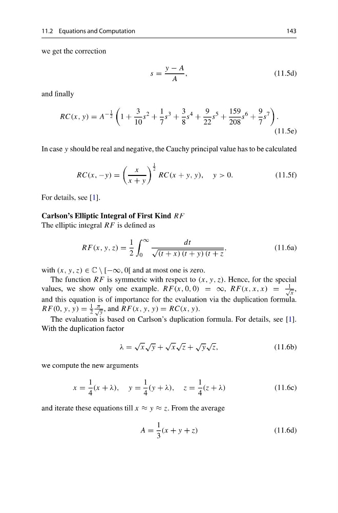
we get the correction
s =
y − A
A
,
(11.5d)
and finally
RC(x, y) = A
−
1
2
1 +
3
10
s
2
+
1
7
s
3
+
3
8
s
4
+
9
22
s
5
+
159
208
s
6
+
9
7
s
7
.
(11.5e)
In case y should be real and negative, the Cauchy principal value has to be calculated
RC(x, −y) =
x
x + y
1
2
RC(x + y, y), y > 0.
(11.5f)
For details, see [1].
Carlson’s Elliptic Integral of First Kind RF
The elliptic integral RF is defined as
RF (x, y, z) =
1
2
∞
0
dt
√
(t + x) (t + y) (t + z
,
(11.6a)
with (x, y, z) ∈ C \ [−∞, 0[ and at most one is zero.
The function RF is symmetric with respect to (x, y, z). Hence, for the special
values, we show only one example. RF (x, 0, 0) = ∞, RF (x, x, x) =
1
√
x
,
and this equation is of importance for the evaluation via the duplication formula.
RF (0, y, y) =
1
2
π
√
y , and RF (x, y, y) = RC(x, y).
The evaluation is based on Carlson’s duplication formula. For details, see [1].
With the duplication factor
λ =
√
x
√
y +
√
x
√
z +
√
y
√
z,
(11.6b)
we compute the new arguments
x =
1
4
(x + λ), y =
1
4
(y + λ), z =
1
4
(z + λ)
(11.6c)
and iterate these equations till x ≈ y ≈ z. From the average
A =
1
3
(x + y + z)
(11.6d)
143
we get the correction
s =
y − A
A
,
(11.5d)
and finally
RC(x, y) = A
−
1
2
1 +
3
10
s
2
+
1
7
s
3
+
3
8
s
4
+
9
22
s
5
+
159
208
s
6
+
9
7
s
7
.
(11.5e)
In case y should be real and negative, the Cauchy principal value has to be calculated
RC(x, −y) =
x
x + y
1
2
RC(x + y, y), y > 0.
(11.5f)
For details, see [1].
Carlson’s Elliptic Integral of First Kind RF
The elliptic integral RF is defined as
RF (x, y, z) =
1
2
∞
0
dt
√
(t + x) (t + y) (t + z
,
(11.6a)
with (x, y, z) ∈ C \ [−∞, 0[ and at most one is zero.
The function RF is symmetric with respect to (x, y, z). Hence, for the special
values, we show only one example. RF (x, 0, 0) = ∞, RF (x, x, x) =
1
√
x
,
and this equation is of importance for the evaluation via the duplication formula.
RF (0, y, y) =
1
2
π
√
y , and RF (x, y, y) = RC(x, y).
The evaluation is based on Carlson’s duplication formula. For details, see [1].
With the duplication factor
λ =
√
x
√
y +
√
x
√
z +
√
y
√
z,
(11.6b)
we compute the new arguments
x =
1
4
(x + λ), y =
1
4
(y + λ), z =
1
4
(z + λ)
(11.6c)
and iterate these equations till x ≈ y ≈ z. From the average
A =
1
3
(x + y + z)
(11.6d)