

142
11 Elliptic Integrals
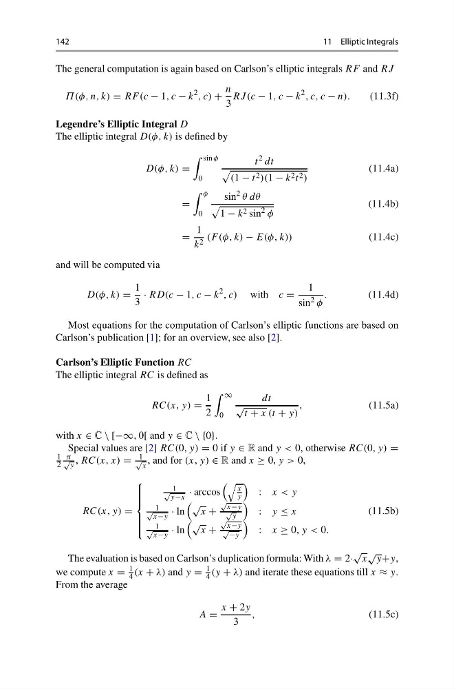
The general computation is again based on Carlson’s elliptic integrals RF and RJ
Π(φ, n, k) = RF (c − 1, c − k
2 , c) +
n
3
RJ (c − 1, c − k
2 , c, c − n).
(11.3f)
Legendre’s Elliptic Integral D
The elliptic integral D(φ, k) is defined by
D(φ, k) =
sin φ
0
t 2 dt
(1 − t 2 )(1 − k 2 t 2 )
(11.4a)
=
φ
0
sin 2 θ dθ
1 − k 2 sin 2 φ
(11.4b)
=
1
k 2 (F (φ, k) − E(φ, k))
(11.4c)
and will be computed via
D(φ, k) =
1
3
· RD(c − 1, c − k
2 , c) with c =
1
sin 2 φ
.
(11.4d)
Most equations for the computation of Carlson’s elliptic functions are based on
Carlson’s publication [1]; for an overview, see also [2].
Carlson’s Elliptic Function RC
The elliptic integral RC is defined as
RC(x, y) =
1
2
∞
0
dt
√
t + x (t + y)
,
(11.5a)
with x ∈ C \ [−∞, 0[ and y ∈ C \ {0}.
Special values are [2] RC(0, y) = 0 if y ∈ R and y < 0, otherwise RC(0, y) =
1
2
π
√ y , RC(x, x) =
1
√
x
, and for (x, y) ∈ R and x ≥ 0, y > 0,
RC(x, y) =
⎧
⎪ ⎪ ⎪ ⎨
⎪ ⎪ ⎪ ⎩
1
√
y−x
· arccos
x
y
: x < y
1
√
x−y
· ln
√
x +
√
x−y
√
y
: y ≤ x
1
√ x−y
· ln
√
x +
√
x−y
√ −y
: x ≥ 0, y < 0.
(11.5b)
The evaluation is based on Carlson’s duplication formula: With λ = 2·
√
x
√ y+y,
we compute x =
1
4 (x + λ) and y =
1
4 (y + λ) and iterate these equations till x ≈ y.
From the average
A =
x + 2y
3
,
(11.5c)
11 Elliptic Integrals
The general computation is again based on Carlson’s elliptic integrals RF and RJ
Π(φ, n, k) = RF (c − 1, c − k
2 , c) +
n
3
RJ (c − 1, c − k
2 , c, c − n).
(11.3f)
Legendre’s Elliptic Integral D
The elliptic integral D(φ, k) is defined by
D(φ, k) =
sin φ
0
t 2 dt
(1 − t 2 )(1 − k 2 t 2 )
(11.4a)
=
φ
0
sin 2 θ dθ
1 − k 2 sin 2 φ
(11.4b)
=
1
k 2 (F (φ, k) − E(φ, k))
(11.4c)
and will be computed via
D(φ, k) =
1
3
· RD(c − 1, c − k
2 , c) with c =
1
sin 2 φ
.
(11.4d)
Most equations for the computation of Carlson’s elliptic functions are based on
Carlson’s publication [1]; for an overview, see also [2].
Carlson’s Elliptic Function RC
The elliptic integral RC is defined as
RC(x, y) =
1
2
∞
0
dt
√
t + x (t + y)
,
(11.5a)
with x ∈ C \ [−∞, 0[ and y ∈ C \ {0}.
Special values are [2] RC(0, y) = 0 if y ∈ R and y < 0, otherwise RC(0, y) =
1
2
π
√ y , RC(x, x) =
1
√
x
, and for (x, y) ∈ R and x ≥ 0, y > 0,
RC(x, y) =
⎧
⎪ ⎪ ⎪ ⎨
⎪ ⎪ ⎪ ⎩
1
√
y−x
· arccos
x
y
: x < y
1
√
x−y
· ln
√
x +
√
x−y
√
y
: y ≤ x
1
√ x−y
· ln
√
x +
√
x−y
√ −y
: x ≥ 0, y < 0.
(11.5b)
The evaluation is based on Carlson’s duplication formula: With λ = 2·
√
x
√ y+y,
we compute x =
1
4 (x + λ) and y =
1
4 (y + λ) and iterate these equations till x ≈ y.
From the average
A =
x + 2y
3
,
(11.5c)