

10.3 The Class ellipFun
137
gives
β
2 (1 + k
2 ) = 1 and β
2 α
2 k
2
=
1
8
,
and thus,
α
2
=
1 ±
√
1 − E
4E
β
2
= 2Eα
2 , and k
2
=
1
8
1
β 2 α 2 ,
and
p(t) =
dx(t)
dt
=
β
α
d sn(βt, k)
d(βt)
.
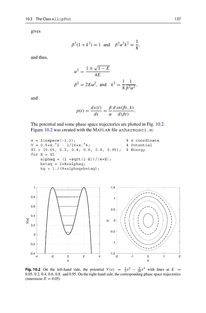
The potential and some phase space trajectories are plotted in Fig. 10.2.
Figure 10.2 was created with the MATLAB file anharmosci.m:
x = linspace(-3,3);
% x coordinate
V = 0.5 * x.^2 - 1/16 * x.^4;
% Potential
El = [0.05, 0.2, 0.4, 0.6, 0.8, 0.95]; % Energy
for E = El
alphaq = (1 +sqrt(1-E))/(4 * E);
betaq = 2 * E * alphaq;
kq = 1./(8 * alphaq * betaq);
-4
-2
0
2
4
x
-0.4
-0.2
0
0.2
0.4
0.6
0.8
1
V(x)
-2
-1
0
1
2
x
-1.5
-1
-0.5
0
0.5
1
1.5
p
Fig. 10.2 On the left-hand side, the potential V (x) =
1
2 x 2 −
1
16 x 4 with lines at E =
0.05, 0.2, 0.4, 0.6, 0.8, and 0.95. On the right-hand side, the corresponding phase space trajectories
(innermost E = 0.05)
137
gives
β
2 (1 + k
2 ) = 1 and β
2 α
2 k
2
=
1
8
,
and thus,
α
2
=
1 ±
√
1 − E
4E
β
2
= 2Eα
2 , and k
2
=
1
8
1
β 2 α 2 ,
and
p(t) =
dx(t)
dt
=
β
α
d sn(βt, k)
d(βt)
.
The potential and some phase space trajectories are plotted in Fig. 10.2.
Figure 10.2 was created with the MATLAB file anharmosci.m:
x = linspace(-3,3);
% x coordinate
V = 0.5 * x.^2 - 1/16 * x.^4;
% Potential
El = [0.05, 0.2, 0.4, 0.6, 0.8, 0.95]; % Energy
for E = El
alphaq = (1 +sqrt(1-E))/(4 * E);
betaq = 2 * E * alphaq;
kq = 1./(8 * alphaq * betaq);
-4
-2
0
2
4
x
-0.4
-0.2
0
0.2
0.4
0.6
0.8
1
V(x)
-2
-1
0
1
2
x
-1.5
-1
-0.5
0
0.5
1
1.5
p
Fig. 10.2 On the left-hand side, the potential V (x) =
1
2 x 2 −
1
16 x 4 with lines at E =
0.05, 0.2, 0.4, 0.6, 0.8, and 0.95. On the right-hand side, the corresponding phase space trajectories
(innermost E = 0.05)