

136
10 Jacobi Elliptic Functions
amplitude function am). “z” is the function variable, e.g., sn(z, k), and could be an
arbitrary complex array, and “k” is the modulus and a complex scalar. The output
“obj” is the class object with the properties “value” (the corresponding function
values), “z” (the input at which the function has been evaluated), “ktau” (the input
modulus k and the corresponding parameter tau as complex vector), and “info” with
some general information including hints with respect to computation.
Examples
(a) Visualizing elliptic functions:
>> k = 0.5;
% modulus
>> x = linspace(-3,3);
>> [X,Y] = meshgrid(x,x);
% complex plane
>> z = X + i * Y;
>> funvalue = ellipFun(’djac’, z, k).value;%fct values
% visualization of sn(z,t)
>> surf(X,Y,abs(funvalue.sn)), shading interp
% visualization of the derivative of sn(z,t)
>> figure, surf(X,Y,abs(funvalue.snd)), shading interp
>> zlim([0,25]), shg
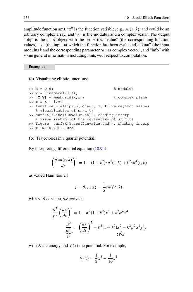
(b) Trajectories in a quartic potential.
By interpreting differential equation (10.9b)
d sn(z, k)
dz
2
= 1 − (1 + k
2 )sn
2 (z, k) + k
2 sn
4 (z, k)
as scaled Hamiltonian
z = βt, x(t) =
1
α
sn(βt, k),
with α, β constant, we arrive at
α 2
β 2
dx
dt
2
= 1 − α
2 (1 + k
2 )x
2
+ k
2 α
4 x
4
β 2
α 2
2E
=
dx
dt
2
+ β
2 (1 + k
2 )x
2
− k
2 β
2 α
2 y
4
2V (x)
,
with E the energy and V (x) the potential. For example,
V (x) =
1
2
x
2
−
1
16
x
4
10 Jacobi Elliptic Functions
amplitude function am). “z” is the function variable, e.g., sn(z, k), and could be an
arbitrary complex array, and “k” is the modulus and a complex scalar. The output
“obj” is the class object with the properties “value” (the corresponding function
values), “z” (the input at which the function has been evaluated), “ktau” (the input
modulus k and the corresponding parameter tau as complex vector), and “info” with
some general information including hints with respect to computation.
Examples
(a) Visualizing elliptic functions:
>> k = 0.5;
% modulus
>> x = linspace(-3,3);
>> [X,Y] = meshgrid(x,x);
% complex plane
>> z = X + i * Y;
>> funvalue = ellipFun(’djac’, z, k).value;%fct values
% visualization of sn(z,t)
>> surf(X,Y,abs(funvalue.sn)), shading interp
% visualization of the derivative of sn(z,t)
>> figure, surf(X,Y,abs(funvalue.snd)), shading interp
>> zlim([0,25]), shg
(b) Trajectories in a quartic potential.
By interpreting differential equation (10.9b)
d sn(z, k)
dz
2
= 1 − (1 + k
2 )sn
2 (z, k) + k
2 sn
4 (z, k)
as scaled Hamiltonian
z = βt, x(t) =
1
α
sn(βt, k),
with α, β constant, we arrive at
α 2
β 2
dx
dt
2
= 1 − α
2 (1 + k
2 )x
2
+ k
2 α
4 x
4
β 2
α 2
2E
=
dx
dt
2
+ β
2 (1 + k
2 )x
2
− k
2 β
2 α
2 y
4
2V (x)
,
with E the energy and V (x) the potential. For example,
V (x) =
1
2
x
2
−
1
16
x
4