

7.2 The Coulomb Wave Functions
103
and thus, [2]
η
d 2
dη 2 + (1 − ikη)
d
dη
− γ k
w(η) = 0,
(7.6)
with the confluent hypergeometric functions 1 F 1 (−iγ ; 1; ik(r − z)), see Eq. (6.3),
as solution of this equation.
7.1
Function Overview
Coulomb Functions: The SPECFUNPHYS class coulombwave supports the
evaluation of the Coulomb wave functions F l , G l , H
±
l , f l , h l , based on a
spherical representation of the Schrödinger equation.
Scattering Functions: The SPECFUNPHYS class coulombscatt allows the
computation of the wave function, corresponding to an incident wave in k,
respectively, z-direction and an outgoing scattering wave. In addition, for convenience, the function rutherford supports the evaluation of the asymptotic
Coulomb scattering amplitude and the Rutherford cross section.
7.2
The Coulomb Wave Functions
7.2.1 Partial Wave Coulomb Function
Spherical Coordinates: Parameterization (a)
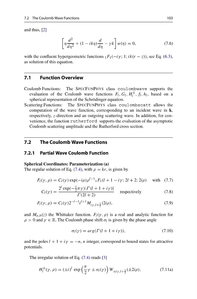
The regular solution of Eq. (7.4), with ρ = kr, is given by
F l (γ , ρ) = C l (γ ) exp(−iρ)ρ
l+1
1 F 1 (l + 1 − iγ ; 2l + 2; 2iρ) with (7.7)
C l (γ ) =
2 l exp(−
1
2 πγ )|Γ (l + 1 + iγ )|
Γ (2l + 2)
respectively
(7.8)
F l (γ , ρ) = C l (γ )2
−l−1 i
l+1 M iγ ,l+
1
2
(2iρ),
(7.9)
and M a,b (z) the Whittaker function. F l (γ , ρ) is a real and analytic function for
ρ > 0 and γ ∈ R. The Coulomb phase shift σ l is given by the phase angle
σ l (γ ) = arg(Γ (l + 1 + iγ )),
(7.10)
and the poles l + 1 + iγ = −n, n integer, correspond to bound states for attractive
potentials.
The irregular solution of Eq. (7.4) reads [3]
H
±
l (γ , ρ) = (±i)
l exp
π
2
γ ± σ l (γ )
W ±iγ ,l+
1
2
(±2iρ),
(7.11a)
103
and thus, [2]
η
d 2
dη 2 + (1 − ikη)
d
dη
− γ k
w(η) = 0,
(7.6)
with the confluent hypergeometric functions 1 F 1 (−iγ ; 1; ik(r − z)), see Eq. (6.3),
as solution of this equation.
7.1
Function Overview
Coulomb Functions: The SPECFUNPHYS class coulombwave supports the
evaluation of the Coulomb wave functions F l , G l , H
±
l , f l , h l , based on a
spherical representation of the Schrödinger equation.
Scattering Functions: The SPECFUNPHYS class coulombscatt allows the
computation of the wave function, corresponding to an incident wave in k,
respectively, z-direction and an outgoing scattering wave. In addition, for convenience, the function rutherford supports the evaluation of the asymptotic
Coulomb scattering amplitude and the Rutherford cross section.
7.2
The Coulomb Wave Functions
7.2.1 Partial Wave Coulomb Function
Spherical Coordinates: Parameterization (a)
The regular solution of Eq. (7.4), with ρ = kr, is given by
F l (γ , ρ) = C l (γ ) exp(−iρ)ρ
l+1
1 F 1 (l + 1 − iγ ; 2l + 2; 2iρ) with (7.7)
C l (γ ) =
2 l exp(−
1
2 πγ )|Γ (l + 1 + iγ )|
Γ (2l + 2)
respectively
(7.8)
F l (γ , ρ) = C l (γ )2
−l−1 i
l+1 M iγ ,l+
1
2
(2iρ),
(7.9)
and M a,b (z) the Whittaker function. F l (γ , ρ) is a real and analytic function for
ρ > 0 and γ ∈ R. The Coulomb phase shift σ l is given by the phase angle
σ l (γ ) = arg(Γ (l + 1 + iγ )),
(7.10)
and the poles l + 1 + iγ = −n, n integer, correspond to bound states for attractive
potentials.
The irregular solution of Eq. (7.4) reads [3]
H
±
l (γ , ρ) = (±i)
l exp
π
2
γ ± σ l (γ )
W ±iγ ,l+
1
2
(±2iρ),
(7.11a)