

88
5 Struve Functions and Related Functions
2
4
6
8
1 0
z
-0.3
-0.2
-0.1
0
0.1
0.2
0.3
0.4
f(z)
2
4
6
8
1 0
z
-0.2
0
0.2
0.4
0.6
0.8
1
1.2
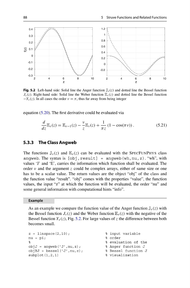
Fig. 5.2 Left-hand side: Solid line the Anger function J ν (z) and dotted line the Bessel function
J ν (z). Right-hand side: Solid line the Weber function E ν (z) and dotted line the Bessel function
−Y ν (z). In all cases the order ν = π, thus far away from being integer
equation (5.20). The first derivative could be evaluated via
d
dz
E ν (z) = E ν−1 (z) −
ν
z
E ν (z) +
1
πz
(1 − cos(πν)) .
(5.21)
5.3.3 The Class Angweb
The functions J ν (z) and E ν (z) can be evaluated with the SPECFUNPHYS class
angweb. The syntax is [obj,result] = angweb(wh,nu,z). “wh”, with
values ‘J’ and ‘E’, carries the information which function shall be evaluated. The
order ν and the argument z could be complex arrays, either of same size or one
has to be a scalar value. The return values are the object “obj” of the class and
the function value “result”. “obj” comes with the properties “value”, the function
values, the input “z” at which the function will be evaluated, the order “nu” and
some general information with computational hints “info”.
Example
As an example we compare the function value of the Anger function J ν (z) with
the Bessel function J ν (z) and the Weber function E ν (z) with the negative of the
Bessel function Y ν (z), Fig. 5.2. For large values of z the difference between both
becomes small.
z = linspace(2,10);
% input variable
nu = pi;
% order
%
% evaluation of the
objJ = angweb(’J’,nu,z);
% Anger function J
objBJ = bessel(’J’,nu,z);
% Bessel function J
subplot(1,2,1)
% visualization
5 Struve Functions and Related Functions
2
4
6
8
1 0
z
-0.3
-0.2
-0.1
0
0.1
0.2
0.3
0.4
f(z)
2
4
6
8
1 0
z
-0.2
0
0.2
0.4
0.6
0.8
1
1.2
Fig. 5.2 Left-hand side: Solid line the Anger function J ν (z) and dotted line the Bessel function
J ν (z). Right-hand side: Solid line the Weber function E ν (z) and dotted line the Bessel function
−Y ν (z). In all cases the order ν = π, thus far away from being integer
equation (5.20). The first derivative could be evaluated via
d
dz
E ν (z) = E ν−1 (z) −
ν
z
E ν (z) +
1
πz
(1 − cos(πν)) .
(5.21)
5.3.3 The Class Angweb
The functions J ν (z) and E ν (z) can be evaluated with the SPECFUNPHYS class
angweb. The syntax is [obj,result] = angweb(wh,nu,z). “wh”, with
values ‘J’ and ‘E’, carries the information which function shall be evaluated. The
order ν and the argument z could be complex arrays, either of same size or one
has to be a scalar value. The return values are the object “obj” of the class and
the function value “result”. “obj” comes with the properties “value”, the function
values, the input “z” at which the function will be evaluated, the order “nu” and
some general information with computational hints “info”.
Example
As an example we compare the function value of the Anger function J ν (z) with
the Bessel function J ν (z) and the Weber function E ν (z) with the negative of the
Bessel function Y ν (z), Fig. 5.2. For large values of z the difference between both
becomes small.
z = linspace(2,10);
% input variable
nu = pi;
% order
%
% evaluation of the
objJ = angweb(’J’,nu,z);
% Anger function J
objBJ = bessel(’J’,nu,z);
% Bessel function J
subplot(1,2,1)
% visualization