

86
5 Struve Functions and Related Functions
0.2
-2
0
0.1
= 1
imag 0
2
real
0
-0.1
-0.2
-0.2
-2
0.04
0
0.02
0.04
= 2
0.02
imag
0
2
real
0
-0.02
-0.02
-0.04
-0.04
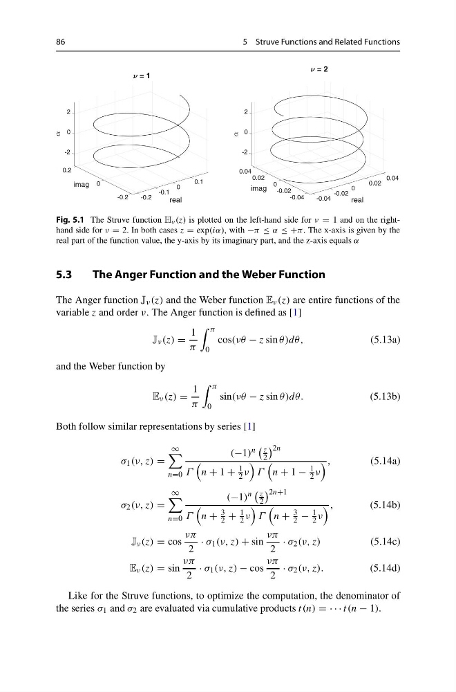
Fig. 5.1 The Struve function H ν (z) is plotted on the left-hand side for ν = 1 and on the righthand side for ν = 2. In both cases z = exp(iα), with −π ≤ α ≤ +π. The x-axis is given by the
real part of the function value, the y-axis by its imaginary part, and the z-axis equals α
5.3
The Anger Function and the Weber Function
The Anger function J ν (z) and the Weber function E ν (z) are entire functions of the
variable z and order ν. The Anger function is defined as [1]
J ν (z) =
1
π
π
0
cos(νθ − z sin θ)dθ,
(5.13a)
and the Weber function by
E ν (z) =
1
π
π
0
sin(νθ − z sin θ)dθ.
(5.13b)
Both follow similar representations by series [1]
σ 1 (ν, z) =
∞
n=0
(−1) n z
2
2n
Γ
n + 1 +
1
2 ν
Γ
n + 1 −
1
2 ν
,
(5.14a)
σ 2 (ν, z) =
∞
n=0
(−1) n z
2
2n+1
Γ
n +
3
2 +
1
2 ν
Γ
n +
3
2 −
1
2 ν
,
(5.14b)
J ν (z) = cos
νπ
2
· σ 1 (ν, z) + sin
νπ
2
· σ 2 (ν, z)
(5.14c)
E ν (z) = sin
νπ
2
· σ 1 (ν, z) − cos
νπ
2
· σ 2 (ν, z).
(5.14d)
Like for the Struve functions, to optimize the computation, the denominator of
the series σ 1 and σ 2 are evaluated via cumulative products t (n) = · · · t (n − 1).
5 Struve Functions and Related Functions
0.2
-2
0
0.1
= 1
imag 0
2
real
0
-0.1
-0.2
-0.2
-2
0.04
0
0.02
0.04
= 2
0.02
imag
0
2
real
0
-0.02
-0.02
-0.04
-0.04
Fig. 5.1 The Struve function H ν (z) is plotted on the left-hand side for ν = 1 and on the righthand side for ν = 2. In both cases z = exp(iα), with −π ≤ α ≤ +π. The x-axis is given by the
real part of the function value, the y-axis by its imaginary part, and the z-axis equals α
5.3
The Anger Function and the Weber Function
The Anger function J ν (z) and the Weber function E ν (z) are entire functions of the
variable z and order ν. The Anger function is defined as [1]
J ν (z) =
1
π
π
0
cos(νθ − z sin θ)dθ,
(5.13a)
and the Weber function by
E ν (z) =
1
π
π
0
sin(νθ − z sin θ)dθ.
(5.13b)
Both follow similar representations by series [1]
σ 1 (ν, z) =
∞
n=0
(−1) n z
2
2n
Γ
n + 1 +
1
2 ν
Γ
n + 1 −
1
2 ν
,
(5.14a)
σ 2 (ν, z) =
∞
n=0
(−1) n z
2
2n+1
Γ
n +
3
2 +
1
2 ν
Γ
n +
3
2 −
1
2 ν
,
(5.14b)
J ν (z) = cos
νπ
2
· σ 1 (ν, z) + sin
νπ
2
· σ 2 (ν, z)
(5.14c)
E ν (z) = sin
νπ
2
· σ 1 (ν, z) − cos
νπ
2
· σ 2 (ν, z).
(5.14d)
Like for the Struve functions, to optimize the computation, the denominator of
the series σ 1 and σ 2 are evaluated via cumulative products t (n) = · · · t (n − 1).