

178
11 Statistics of Counting
(σ u )
2
= (σ x )
2
+ (σ y )
2
(11.2)
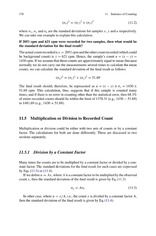
where σ x , σ y and σ u are the standard deviations for samples x, y and u respectively.
We can take one example to explain this calculation.
If 2051 cpm and 621 cpm were recorded for two samples, then what would be
the standard deviation for the final result?
The actual count recorded is x = 2051 cpm and the other count recorded (which could
be background count) is y = 621 cpm. Hence, the sample’s count u = (x − y) =
1430 cpm. If we assume that these counts are approximately equal to mean (because
normally we do not carry out the measurements several times to calculate the mean
count), we can calculate the standard deviation of the final result as follows:
(σ u )
2
= (σ x )
2
+ (σ y )
2
= 51.69
The final result should, therefore, be represented as u = (x − y) ± σ y = 1430 ±
51.69 cpm. This calculation, thus, suggests that if this sample is counted many
times, and if there is no error in counting other than the statistical error, then 68.3%
of entire recorded counts should lie within the limit of 1378.31 (e.g., 1430 − 51.69)
to 1481.69 (e.g., 1430 + 51.69).
11.5 Multiplication or Division to Recorded Count
Multiplication or division could be either with two sets of counts or by a constant
factor. The calculations for both are done differently. These are discussed in two
sections separately.
11.5.1 Division by a Constant Factor
Many times the counts are to be multiplied by a constant factor or divided by a constant factor. The standard deviations for the final result for such cases are expressed
by Eqs. (11.3) or (11.4).
If we define u = Ax, where A is a constant factor to be multiplied by the observed
count x, then the standard deviation of the final result is given by Eq. (11.3)
σ u = Aσ x
(11.3)
In other case, where u = x/A, i.e., the count x is divided by a constant factor A,
then the standard deviation of the final result is given by Eq. (11.4).
11 Statistics of Counting
(σ u )
2
= (σ x )
2
+ (σ y )
2
(11.2)
where σ x , σ y and σ u are the standard deviations for samples x, y and u respectively.
We can take one example to explain this calculation.
If 2051 cpm and 621 cpm were recorded for two samples, then what would be
the standard deviation for the final result?
The actual count recorded is x = 2051 cpm and the other count recorded (which could
be background count) is y = 621 cpm. Hence, the sample’s count u = (x − y) =
1430 cpm. If we assume that these counts are approximately equal to mean (because
normally we do not carry out the measurements several times to calculate the mean
count), we can calculate the standard deviation of the final result as follows:
(σ u )
2
= (σ x )
2
+ (σ y )
2
= 51.69
The final result should, therefore, be represented as u = (x − y) ± σ y = 1430 ±
51.69 cpm. This calculation, thus, suggests that if this sample is counted many
times, and if there is no error in counting other than the statistical error, then 68.3%
of entire recorded counts should lie within the limit of 1378.31 (e.g., 1430 − 51.69)
to 1481.69 (e.g., 1430 + 51.69).
11.5 Multiplication or Division to Recorded Count
Multiplication or division could be either with two sets of counts or by a constant
factor. The calculations for both are done differently. These are discussed in two
sections separately.
11.5.1 Division by a Constant Factor
Many times the counts are to be multiplied by a constant factor or divided by a constant factor. The standard deviations for the final result for such cases are expressed
by Eqs. (11.3) or (11.4).
If we define u = Ax, where A is a constant factor to be multiplied by the observed
count x, then the standard deviation of the final result is given by Eq. (11.3)
σ u = Aσ x
(11.3)
In other case, where u = x/A, i.e., the count x is divided by a constant factor A,
then the standard deviation of the final result is given by Eq. (11.4).