

174
11 Statistics of Counting
may not be a true representation of count. Then how do we represent the count such
that no matter who makes the measurement, one would be able to get a similar count.
For this purpose, we take the help of Gaussian distribution Law.
11.3 Gaussian Distribution Curve
When the number of events recorded in any measurement is of random nature,
as is the case with radioactivity measurements, one takes the help of
Gaussian distribution law; which suggests that if the measurements of counts follow
purely statistical variation, then the distribution of counts should follow a symmetrical distribution around its mean value (Fig. 11.1). This graph is plotted from the
experimental results of Table 11.2. Various useful information can be derived from
this distribution curve. Before we discuss its application, it is necessary we educate
ourselves with a term called standard deviation.
11.3.1 Standard Deviation
Normally, one tends to believe that the average of the count can be considered as an
accurate way of representing a data. But this has a serious drawback, which can be
perceived from the graph shown in Fig. 11.1 and the previous example of a family
which wished to cross the river and found all members drowned except the leader
of the family. Therefore, while representing a data, it is advisable to represent the
variation in the mean value also, which is normally done by calculating the standard
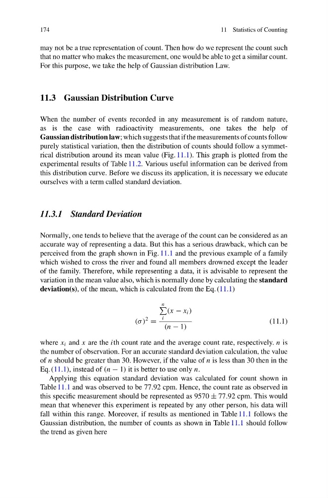
deviation(s), of the mean, which is calculated from the Eq. (11.1)
(σ )
2
=
n
i
(x − x i )
(n − 1)
(11.1)
where x i and x are the ith count rate and the average count rate, respectively. n is
the number of observation. For an accurate standard deviation calculation, the value
of n should be greater than 30. However, if the value of n is less than 30 then in the
Eq. (11.1), instead of (n − 1) it is better to use only n.
Applying this equation standard deviation was calculated for count shown in
Table 11.1 and was observed to be 77.92 cpm. Hence, the count rate as observed in
this specific measurement should be represented as 9570 ± 77.92 cpm. This would
mean that whenever this experiment is repeated by any other person, his data will
fall within this range. Moreover, if results as mentioned in Table 11.1 follows the
Gaussian distribution, the number of counts as shown in Table 11.1 should follow
the trend as given here
11 Statistics of Counting
may not be a true representation of count. Then how do we represent the count such
that no matter who makes the measurement, one would be able to get a similar count.
For this purpose, we take the help of Gaussian distribution Law.
11.3 Gaussian Distribution Curve
When the number of events recorded in any measurement is of random nature,
as is the case with radioactivity measurements, one takes the help of
Gaussian distribution law; which suggests that if the measurements of counts follow
purely statistical variation, then the distribution of counts should follow a symmetrical distribution around its mean value (Fig. 11.1). This graph is plotted from the
experimental results of Table 11.2. Various useful information can be derived from
this distribution curve. Before we discuss its application, it is necessary we educate
ourselves with a term called standard deviation.
11.3.1 Standard Deviation
Normally, one tends to believe that the average of the count can be considered as an
accurate way of representing a data. But this has a serious drawback, which can be
perceived from the graph shown in Fig. 11.1 and the previous example of a family
which wished to cross the river and found all members drowned except the leader
of the family. Therefore, while representing a data, it is advisable to represent the
variation in the mean value also, which is normally done by calculating the standard
deviation(s), of the mean, which is calculated from the Eq. (11.1)
(σ )
2
=
n
i
(x − x i )
(n − 1)
(11.1)
where x i and x are the ith count rate and the average count rate, respectively. n is
the number of observation. For an accurate standard deviation calculation, the value
of n should be greater than 30. However, if the value of n is less than 30 then in the
Eq. (11.1), instead of (n − 1) it is better to use only n.
Applying this equation standard deviation was calculated for count shown in
Table 11.1 and was observed to be 77.92 cpm. Hence, the count rate as observed in
this specific measurement should be represented as 9570 ± 77.92 cpm. This would
mean that whenever this experiment is repeated by any other person, his data will
fall within this range. Moreover, if results as mentioned in Table 11.1 follows the
Gaussian distribution, the number of counts as shown in Table 11.1 should follow
the trend as given here