

11.2 Statistical Error in Counting
173
Table 11.2 The distribution counts as recorded in Table 11.1
Range of counts
Number of times it appears
9550–9600
2
9601–9649
3
9650–9700
3
9701–9749
11
9750–9800
13
9801–9849
5
9850–9800
1
9801–9849
1
9900 cpm) and minimum count rate 9600 cpm, we create a set of range as given
in Table 11.1. We find out from Table 11.1 the number of counts appearing in each
of these ranges (known as the frequency of number appearing in the range). These
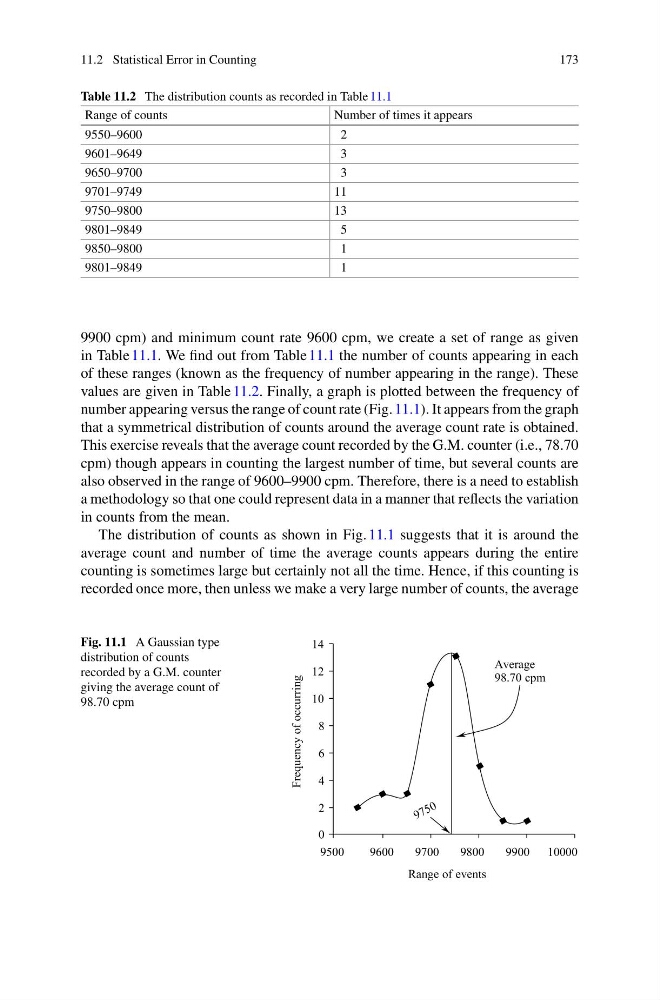
values are given in Table 11.2. Finally, a graph is plotted between the frequency of
number appearing versus the range of count rate (Fig. 11.1). It appears from the graph
that a symmetrical distribution of counts around the average count rate is obtained.
This exercise reveals that the average count recorded by the G.M. counter (i.e., 78.70
cpm) though appears in counting the largest number of time, but several counts are
also observed in the range of 9600–9900 cpm. Therefore, there is a need to establish
a methodology so that one could represent data in a manner that reflects the variation
in counts from the mean.
The distribution of counts as shown in Fig. 11.1 suggests that it is around the
average count and number of time the average counts appears during the entire
counting is sometimes large but certainly not all the time. Hence, if this counting is
recorded once more, then unless we make a very large number of counts, the average
Fig. 11.1 A Gaussian type
distribution of counts
recorded by a G.M. counter
giving the average count of
98.70 cpm
14
12
10
8
6
4
2
0
9500
9600
9700
9800
9900 10000
Range of events
Frequency of occurring
9 7 5 0
Average
98.70 cpm
173
Table 11.2 The distribution counts as recorded in Table 11.1
Range of counts
Number of times it appears
9550–9600
2
9601–9649
3
9650–9700
3
9701–9749
11
9750–9800
13
9801–9849
5
9850–9800
1
9801–9849
1
9900 cpm) and minimum count rate 9600 cpm, we create a set of range as given
in Table 11.1. We find out from Table 11.1 the number of counts appearing in each
of these ranges (known as the frequency of number appearing in the range). These
values are given in Table 11.2. Finally, a graph is plotted between the frequency of
number appearing versus the range of count rate (Fig. 11.1). It appears from the graph
that a symmetrical distribution of counts around the average count rate is obtained.
This exercise reveals that the average count recorded by the G.M. counter (i.e., 78.70
cpm) though appears in counting the largest number of time, but several counts are
also observed in the range of 9600–9900 cpm. Therefore, there is a need to establish
a methodology so that one could represent data in a manner that reflects the variation
in counts from the mean.
The distribution of counts as shown in Fig. 11.1 suggests that it is around the
average count and number of time the average counts appears during the entire
counting is sometimes large but certainly not all the time. Hence, if this counting is
recorded once more, then unless we make a very large number of counts, the average
Fig. 11.1 A Gaussian type
distribution of counts
recorded by a G.M. counter
giving the average count of
98.70 cpm
14
12
10
8
6
4
2
0
9500
9600
9700
9800
9900 10000
Range of events
Frequency of occurring
9 7 5 0
Average
98.70 cpm