

2 General Relativity Measurements from Pulsars
77
simple timing model including a minimal set of pulsar parameters (approximate
spin period, DM and position). We then create timing residuals by comparing the
observed ToAs with ToAs predicted on the basis of our model and we plot the
residual as a function of time. We then search for trends in the timing residuals and
fit for the model parameter(s) that can account for the trend(s) observed: a linear
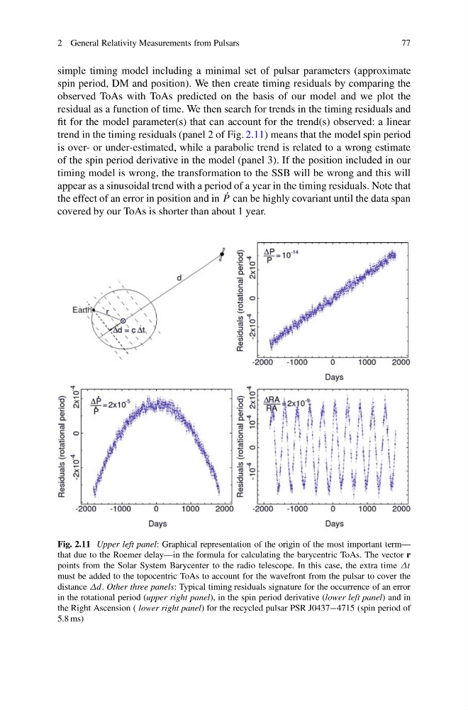
trend in the timing residuals (panel 2 of Fig. 2.11) means that the model spin period
is over- or under-estimated, while a parabolic trend is related to a wrong estimate
of the spin period derivative in the model (panel 3). If the position included in our
timing model is wrong, the transformation to the SSB will be wrong and this will
appear as a sinusoidal trend with a period of a year in the timing residuals. Note that
the effect of an error in position and in ˙
P can be highly covariant until the data span
covered by our ToAs is shorter than about 1 year.
Fig. 2.11 Upper left panel: Graphical representation of the origin of the most important term—
that due to the Roemer delay—in the formula for calculating the barycentric ToAs. The vector r
points from the Solar System Barycenter to the radio telescope. In this case, the extra time Δt
must be added to the topocentric ToAs to account for the wavefront from the pulsar to cover the
distance Δd. Other three panels: Typical timing residuals signature for the occurrence of an error
in the rotational period (upper right panel), in the spin period derivative (lower left panel) and in
the Right Ascension ( lower right panel) for the recycled pulsar PSR J0437−4715 (spin period of
5.8 ms)
77
simple timing model including a minimal set of pulsar parameters (approximate
spin period, DM and position). We then create timing residuals by comparing the
observed ToAs with ToAs predicted on the basis of our model and we plot the
residual as a function of time. We then search for trends in the timing residuals and
fit for the model parameter(s) that can account for the trend(s) observed: a linear
trend in the timing residuals (panel 2 of Fig. 2.11) means that the model spin period
is over- or under-estimated, while a parabolic trend is related to a wrong estimate
of the spin period derivative in the model (panel 3). If the position included in our
timing model is wrong, the transformation to the SSB will be wrong and this will
appear as a sinusoidal trend with a period of a year in the timing residuals. Note that
the effect of an error in position and in ˙
P can be highly covariant until the data span
covered by our ToAs is shorter than about 1 year.
Fig. 2.11 Upper left panel: Graphical representation of the origin of the most important term—
that due to the Roemer delay—in the formula for calculating the barycentric ToAs. The vector r
points from the Solar System Barycenter to the radio telescope. In this case, the extra time Δt
must be added to the topocentric ToAs to account for the wavefront from the pulsar to cover the
distance Δd. Other three panels: Typical timing residuals signature for the occurrence of an error
in the rotational period (upper right panel), in the spin period derivative (lower left panel) and in
the Right Ascension ( lower right panel) for the recycled pulsar PSR J0437−4715 (spin period of
5.8 ms)