

280
M. Méndez and T. M. Belloni
30.0
20.0
10.0
0.0
Energy (keV)
0.0
5.0
10.0
15.0
20.0
25.0
30.0
RMS Amplitude of QPO (%)
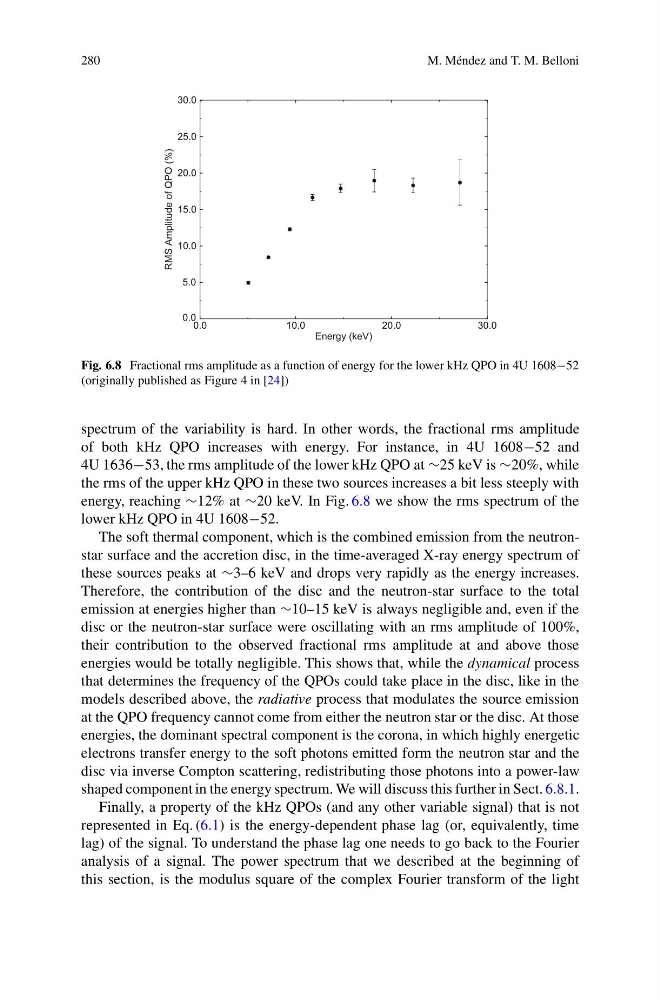
Fig. 6.8 Fractional rms amplitude as a function of energy for the lower kHz QPO in 4U 1608−52
(originally published as Figure 4 in [24])
spectrum of the variability is hard. In other words, the fractional rms amplitude
of both kHz QPO increases with energy. For instance, in 4U 1608−52 and
4U 1636−53, the rms amplitude of the lower kHz QPO at ∼25 keV is ∼20%, while
the rms of the upper kHz QPO in these two sources increases a bit less steeply with
energy, reaching ∼12% at ∼20 keV. In Fig. 6.8 we show the rms spectrum of the
lower kHz QPO in 4U 1608−52.
The soft thermal component, which is the combined emission from the neutronstar surface and the accretion disc, in the time-averaged X-ray energy spectrum of
these sources peaks at ∼3–6 keV and drops very rapidly as the energy increases.
Therefore, the contribution of the disc and the neutron-star surface to the total
emission at energies higher than ∼10–15 keV is always negligible and, even if the
disc or the neutron-star surface were oscillating with an rms amplitude of 100%,
their contribution to the observed fractional rms amplitude at and above those
energies would be totally negligible. This shows that, while the dynamical process
that determines the frequency of the QPOs could take place in the disc, like in the
models described above, the radiative process that modulates the source emission
at the QPO frequency cannot come from either the neutron star or the disc. At those
energies, the dominant spectral component is the corona, in which highly energetic
electrons transfer energy to the soft photons emitted form the neutron star and the
disc via inverse Compton scattering, redistributing those photons into a power-law
shaped component in the energy spectrum. We will discuss this further in Sect. 6.8.1.
Finally, a property of the kHz QPOs (and any other variable signal) that is not
represented in Eq. (6.1) is the energy-dependent phase lag (or, equivalently, time
lag) of the signal. To understand the phase lag one needs to go back to the Fourier
analysis of a signal. The power spectrum that we described at the beginning of
this section, is the modulus square of the complex Fourier transform of the light
M. Méndez and T. M. Belloni
30.0
20.0
10.0
0.0
Energy (keV)
0.0
5.0
10.0
15.0
20.0
25.0
30.0
RMS Amplitude of QPO (%)
Fig. 6.8 Fractional rms amplitude as a function of energy for the lower kHz QPO in 4U 1608−52
(originally published as Figure 4 in [24])
spectrum of the variability is hard. In other words, the fractional rms amplitude
of both kHz QPO increases with energy. For instance, in 4U 1608−52 and
4U 1636−53, the rms amplitude of the lower kHz QPO at ∼25 keV is ∼20%, while
the rms of the upper kHz QPO in these two sources increases a bit less steeply with
energy, reaching ∼12% at ∼20 keV. In Fig. 6.8 we show the rms spectrum of the
lower kHz QPO in 4U 1608−52.
The soft thermal component, which is the combined emission from the neutronstar surface and the accretion disc, in the time-averaged X-ray energy spectrum of
these sources peaks at ∼3–6 keV and drops very rapidly as the energy increases.
Therefore, the contribution of the disc and the neutron-star surface to the total
emission at energies higher than ∼10–15 keV is always negligible and, even if the
disc or the neutron-star surface were oscillating with an rms amplitude of 100%,
their contribution to the observed fractional rms amplitude at and above those
energies would be totally negligible. This shows that, while the dynamical process
that determines the frequency of the QPOs could take place in the disc, like in the
models described above, the radiative process that modulates the source emission
at the QPO frequency cannot come from either the neutron star or the disc. At those
energies, the dominant spectral component is the corona, in which highly energetic
electrons transfer energy to the soft photons emitted form the neutron star and the
disc via inverse Compton scattering, redistributing those photons into a power-law
shaped component in the energy spectrum. We will discuss this further in Sect. 6.8.1.
Finally, a property of the kHz QPOs (and any other variable signal) that is not
represented in Eq. (6.1) is the energy-dependent phase lag (or, equivalently, time
lag) of the signal. To understand the phase lag one needs to go back to the Fourier
analysis of a signal. The power spectrum that we described at the beginning of
this section, is the modulus square of the complex Fourier transform of the light