

232
D. K. Galloway and L. Keek
0
1
1
5
2
0.1
1
10
Flux [phot cm −2
s −1
keV −1
]
Energy [keV]
0
1
1
0
2
5
2
10 −3
0.01
0.1
1
10
[Photons cm −2
s −1
keV −1
]
Energy [keV]
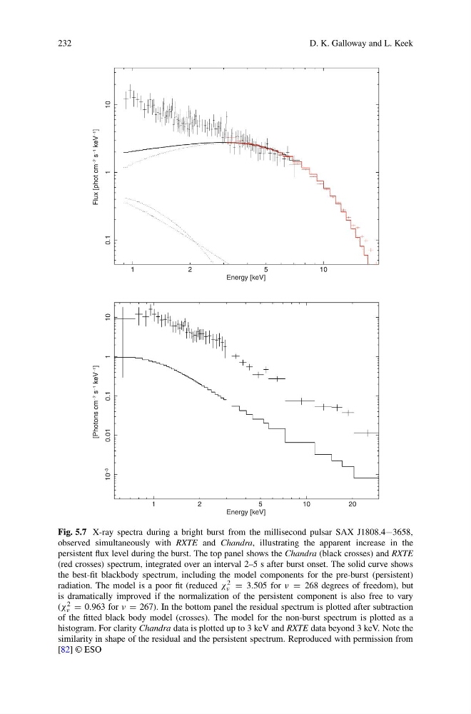
Fig. 5.7 X-ray spectra during a bright burst from the millisecond pulsar SAX J1808.4−3658,
observed simultaneously with RXTE and Chandra, illustrating the apparent increase in the
persistent flux level during the burst. The top panel shows the Chandra (black crosses) and RXTE
(red crosses) spectrum, integrated over an interval 2–5 s after burst onset. The solid curve shows
the best-fit blackbody spectrum, including the model components for the pre-burst (persistent)
radiation. The model is a poor fit (reduced χ 2
ν = 3.505 for ν = 268 degrees of freedom), but
is dramatically improved if the normalization of the persistent component is also free to vary
(χ 2
ν = 0.963 for ν = 267). In the bottom panel the residual spectrum is plotted after subtraction
of the fitted black body model (crosses). The model for the non-burst spectrum is plotted as a
histogram. For clarity Chandra data is plotted up to 3 keV and RXTE data beyond 3 keV. Note the
similarity in shape of the residual and the persistent spectrum. Reproduced with permission from
[82] © ESO
D. K. Galloway and L. Keek
0
1
1
5
2
0.1
1
10
Flux [phot cm −2
s −1
keV −1
]
Energy [keV]
0
1
1
0
2
5
2
10 −3
0.01
0.1
1
10
[Photons cm −2
s −1
keV −1
]
Energy [keV]
Fig. 5.7 X-ray spectra during a bright burst from the millisecond pulsar SAX J1808.4−3658,
observed simultaneously with RXTE and Chandra, illustrating the apparent increase in the
persistent flux level during the burst. The top panel shows the Chandra (black crosses) and RXTE
(red crosses) spectrum, integrated over an interval 2–5 s after burst onset. The solid curve shows
the best-fit blackbody spectrum, including the model components for the pre-burst (persistent)
radiation. The model is a poor fit (reduced χ 2
ν = 3.505 for ν = 268 degrees of freedom), but
is dramatically improved if the normalization of the persistent component is also free to vary
(χ 2
ν = 0.963 for ν = 267). In the bottom panel the residual spectrum is plotted after subtraction
of the fitted black body model (crosses). The model for the non-burst spectrum is plotted as a
histogram. For clarity Chandra data is plotted up to 3 keV and RXTE data beyond 3 keV. Note the
similarity in shape of the residual and the persistent spectrum. Reproduced with permission from
[82] © ESO