

4 Accreting Millisecond X-ray Pulsars
173
frame to the Solar System barycenter (an approximate inertial reference frame)
and correcting for general and special relativistic perturbations due to planets and
minor bodies in the Solar System that affect photon propagation. Before discussing
observational tests of accretion theory it is useful to clarify the observables that play
a role in coherent timing studies. AMXPs show pulsations that are too weak to detect
as single pulses: to reconstruct the signal it is necessary to fold the data in segments
of several hundred seconds to obtain a pulse profile that is the average of several
hundred thousand NS cycles. It is then possible to measure the fractional amplitude
of the pulsations, and the pulse phase. Pulse profiles of AMXPs are generally highly
sinusoidal, with little or no harmonic content beyond the fundamental frequency.
In this case the pulse phases can be measured by choosing a fiducial point (e.g.
the pulse peak) and tracking the variation of the phase at this point over time.
Sometimes, however, strong harmonic content is observed, with the pulse profile
shape varying during an outburst. This means that unlike in radio pulsar timing,
where average profiles are often very stable, there is no stable fiducial point on
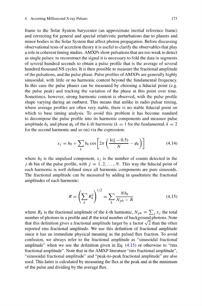
which to base timing analysis. To avoid this problem it has become standard
to decompose the pulse profile into its harmonic components and measure pulse
amplitude b k and phase φ k of the k-th harmonic (k = 1 for the fundamental, k = 2
for the second harmonic and so on) via the expression:
x j = b 0 +
k
b k cos
2π
k(j − 0.5)
N
− φ k
(4.14)
where b 0 is the unpulsed component, x j is the number of counts detected in the
j -th bin of the pulse profile, with j = 1, 2, . . . , N. This way the fiducial point of
each harmonic is well defined since all harmonic components are pure sinusoids.
The fractional amplitude can be measured by adding in quadrature the fractional
amplitudes of each harmonic:
R =
k
R
2
k
1/2
=
k
Nb k
N ph − B
(4.15)
where R k is the fractional amplitude of the k-th harmonic, N ph =
j x j the total
number of photons in a profile and B the total number of background photons. Note
that this definition gives a fractional amplitude larger by a factor
√
2 than the often
reported rms fractional amplitude. We use this definition of fractional amplitude
since it has an immediate physical meaning as the pulsed flux fraction. To avoid
confusion, we always refer to the fractional amplitude as “sinusoidal fractional
amplitude” when we use the definition given in Eq. (4.15) or otherwise to “rms
fractional amplitude”. Note that in the AMXP literature “rms fractional amplitude”,
“sinusoidal fractional amplitude” and “peak-to-peak fractional amplitude” are also
used. This latter is calculated by measuring the flux at the peak and at the minimum
of the pulse and dividing by the average flux.
173
frame to the Solar System barycenter (an approximate inertial reference frame)
and correcting for general and special relativistic perturbations due to planets and
minor bodies in the Solar System that affect photon propagation. Before discussing
observational tests of accretion theory it is useful to clarify the observables that play
a role in coherent timing studies. AMXPs show pulsations that are too weak to detect
as single pulses: to reconstruct the signal it is necessary to fold the data in segments
of several hundred seconds to obtain a pulse profile that is the average of several
hundred thousand NS cycles. It is then possible to measure the fractional amplitude
of the pulsations, and the pulse phase. Pulse profiles of AMXPs are generally highly
sinusoidal, with little or no harmonic content beyond the fundamental frequency.
In this case the pulse phases can be measured by choosing a fiducial point (e.g.
the pulse peak) and tracking the variation of the phase at this point over time.
Sometimes, however, strong harmonic content is observed, with the pulse profile
shape varying during an outburst. This means that unlike in radio pulsar timing,
where average profiles are often very stable, there is no stable fiducial point on
which to base timing analysis. To avoid this problem it has become standard
to decompose the pulse profile into its harmonic components and measure pulse
amplitude b k and phase φ k of the k-th harmonic (k = 1 for the fundamental, k = 2
for the second harmonic and so on) via the expression:
x j = b 0 +
k
b k cos
2π
k(j − 0.5)
N
− φ k
(4.14)
where b 0 is the unpulsed component, x j is the number of counts detected in the
j -th bin of the pulse profile, with j = 1, 2, . . . , N. This way the fiducial point of
each harmonic is well defined since all harmonic components are pure sinusoids.
The fractional amplitude can be measured by adding in quadrature the fractional
amplitudes of each harmonic:
R =
k
R
2
k
1/2
=
k
Nb k
N ph − B
(4.15)
where R k is the fractional amplitude of the k-th harmonic, N ph =
j x j the total
number of photons in a profile and B the total number of background photons. Note
that this definition gives a fractional amplitude larger by a factor
√
2 than the often
reported rms fractional amplitude. We use this definition of fractional amplitude
since it has an immediate physical meaning as the pulsed flux fraction. To avoid
confusion, we always refer to the fractional amplitude as “sinusoidal fractional
amplitude” when we use the definition given in Eq. (4.15) or otherwise to “rms
fractional amplitude”. Note that in the AMXP literature “rms fractional amplitude”,
“sinusoidal fractional amplitude” and “peak-to-peak fractional amplitude” are also
used. This latter is calculated by measuring the flux at the peak and at the minimum
of the pulse and dividing by the average flux.