

Appendix: All Solutions to the Problems
967
= ∇ · [(B · ∇a) · δa] − [∇ · (B · ∇a)] · δa
+ [δa · (a∇ · B)] · ∇ − [(a∇ · B) · ∇] · δa
(5)
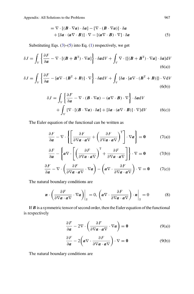
Substituting Eqs. (3)–(5) into Eq. (1) respectively, we get
δ J =
V
∂ F
∂ a
− ∇ · [(B + B
T
) · ∇a]
· δadV +
V
∇ · {[(B + B
T
) · ∇a] · δa}dV
(6(a))
δ J =
V
∂ F
∂ a
− [a∇ · (B
T
+ B)] · ∇
· δadV +
V
{δa · [a∇ · (B
T
+ B)]} · ∇dV
(6(b))
δ J =
V
∂ F
∂ a
− ∇ · (B · ∇a) − (a∇ · B) · ∇
· δadV
+
V
{∇ · [(B · ∇a) · δa] + [δa · (a∇ · B)] · ∇}dV
(6(c))
The Euler equation of the functional can be written as
∂ F
∂ a
− ∇ ·
∂ F
∂∇ a · a∇
+
∂ F
∂∇ a · a∇
T
· ∇a
= 0
(7(a))
∂ F
∂ a
−
a∇ ·
∂ F
∂∇ a · a∇
T
+
∂ F
∂∇ a · a∇
· ∇ = 0
(7(b))
∂ F
∂ a
− ∇ ·
∂ F
∂∇ a · a∇
· ∇a
−
a∇ ·
∂ F
∂∇ a · a∇
· ∇ = 0
(7(c))
The natural boundary conditions are
n ·
∂ F
∂∇ a · a∇
· ∇a
S
= 0,
a∇ ·
∂ F
∂∇ a · a∇
· n
S
= 0
( 8 )
If B is a symmetric tensor of second order, then the Euler equation of the functional
is respectively
∂ F
∂ a
− 2∇ ·
∂ F
∂∇ a · a∇
· ∇a
= 0
(9(a))
∂ F
∂ a
− 2
a∇ ·
∂ F
∂∇ a · a∇
· ∇ = 0
(9(b))
The natural boundary conditions are
967
= ∇ · [(B · ∇a) · δa] − [∇ · (B · ∇a)] · δa
+ [δa · (a∇ · B)] · ∇ − [(a∇ · B) · ∇] · δa
(5)
Substituting Eqs. (3)–(5) into Eq. (1) respectively, we get
δ J =
V
∂ F
∂ a
− ∇ · [(B + B
T
) · ∇a]
· δadV +
V
∇ · {[(B + B
T
) · ∇a] · δa}dV
(6(a))
δ J =
V
∂ F
∂ a
− [a∇ · (B
T
+ B)] · ∇
· δadV +
V
{δa · [a∇ · (B
T
+ B)]} · ∇dV
(6(b))
δ J =
V
∂ F
∂ a
− ∇ · (B · ∇a) − (a∇ · B) · ∇
· δadV
+
V
{∇ · [(B · ∇a) · δa] + [δa · (a∇ · B)] · ∇}dV
(6(c))
The Euler equation of the functional can be written as
∂ F
∂ a
− ∇ ·
∂ F
∂∇ a · a∇
+
∂ F
∂∇ a · a∇
T
· ∇a
= 0
(7(a))
∂ F
∂ a
−
a∇ ·
∂ F
∂∇ a · a∇
T
+
∂ F
∂∇ a · a∇
· ∇ = 0
(7(b))
∂ F
∂ a
− ∇ ·
∂ F
∂∇ a · a∇
· ∇a
−
a∇ ·
∂ F
∂∇ a · a∇
· ∇ = 0
(7(c))
The natural boundary conditions are
n ·
∂ F
∂∇ a · a∇
· ∇a
S
= 0,
a∇ ·
∂ F
∂∇ a · a∇
· n
S
= 0
( 8 )
If B is a symmetric tensor of second order, then the Euler equation of the functional
is respectively
∂ F
∂ a
− 2∇ ·
∂ F
∂∇ a · a∇
· ∇a
= 0
(9(a))
∂ F
∂ a
− 2
a∇ ·
∂ F
∂∇ a · a∇
· ∇ = 0
(9(b))
The natural boundary conditions are