

956
Appendix: All Solutions to the Problems
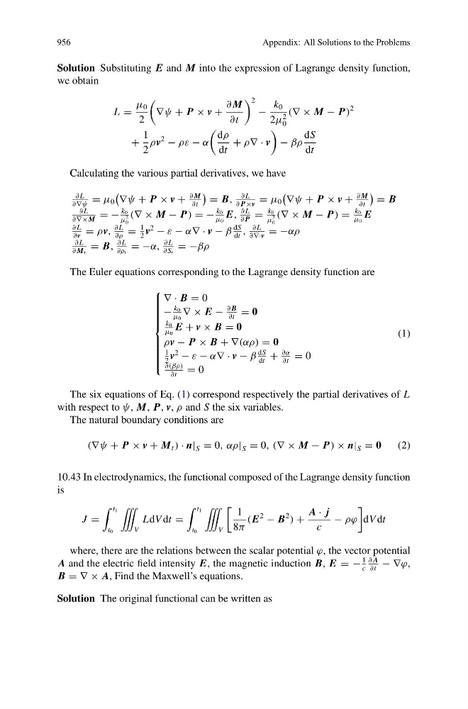
Solution Substituting E and M into the expression of Lagrange density function,
we obtain
L =
μ 0
2
∇ψ + P × v +
∂ M
∂t
2
−
k 0
2μ
2
0
(∇ × M − P)
2
+
1
2
ρv
2
− ρε − α
dρ
dt
+ ρ∇ · v
− βρ
dS
dt
Calculating the various partial derivatives, we have
∂ L
∂∇ψ
= μ 0
∇ψ + P × v +
∂ M
∂t
= B,
∂ L
∂ P×v
= μ 0
∇ψ + P × v +
∂ M
∂t
= B
∂ L
∂∇×M
= −
k 0
μ
2
0
(∇ × M − P) = −
k 0
μ 0
E,
∂ L
∂ P
=
k 0
μ
2
0
(∇ × M − P) =
k 0
μ 0
E
∂ L
∂v
= ρv,
∂ L
∂ρ
=
1
2
v
2
− ε − α∇ · v − β
dS
dt
,
∂ L
∂∇·v
= −αρ
∂ L
∂ M t
= B,
∂ L
∂ρ t
= −α,
∂ L
∂ S t
= −βρ
The Euler equations corresponding to the Lagrange density function are
⎧
⎪ ⎪ ⎪ ⎪ ⎪ ⎪ ⎪ ⎨
⎪ ⎪ ⎪ ⎪ ⎪ ⎪ ⎪ ⎩
∇ · B = 0
−
k 0
μ 0
∇ × E −
∂ B
∂t
= 0
k 0
μ 0
E + v × B = 0
ρv − P × B + ∇(αρ) = 0
1
2
v
2
− ε − α∇ · v − β
dS
dt
+
∂α
∂t
= 0
∂(βρ)
∂t
= 0
(1)
The six equations of Eq. (1) correspond respectively the partial derivatives of L
with respect to ψ, M, P, v, ρ and S the six variables.
The natural boundary conditions are
(∇ψ + P × v + M t ) · n| S = 0, αρ| S = 0, (∇ × M − P) × n| S = 0
(2)
10.43 In electrodynamics, the functional composed of the Lagrange density function
is
J =
t 1
t 0
˚
V
LdV dt =
t 1
t 0
˚
V
1
8π
(E
2
− B
2
) +
A · j
c
− ρϕ
dV dt
where, there are the relations between the scalar potential ϕ, the vector potential
A and the electric field intensity E, the magnetic induction B, E = −
1
c
∂ A
∂t
− ∇ϕ,
B = ∇ × A, Find the Maxwell’s equations.
Solution The original functional can be written as
Appendix: All Solutions to the Problems
Solution Substituting E and M into the expression of Lagrange density function,
we obtain
L =
μ 0
2
∇ψ + P × v +
∂ M
∂t
2
−
k 0
2μ
2
0
(∇ × M − P)
2
+
1
2
ρv
2
− ρε − α
dρ
dt
+ ρ∇ · v
− βρ
dS
dt
Calculating the various partial derivatives, we have
∂ L
∂∇ψ
= μ 0
∇ψ + P × v +
∂ M
∂t
= B,
∂ L
∂ P×v
= μ 0
∇ψ + P × v +
∂ M
∂t
= B
∂ L
∂∇×M
= −
k 0
μ
2
0
(∇ × M − P) = −
k 0
μ 0
E,
∂ L
∂ P
=
k 0
μ
2
0
(∇ × M − P) =
k 0
μ 0
E
∂ L
∂v
= ρv,
∂ L
∂ρ
=
1
2
v
2
− ε − α∇ · v − β
dS
dt
,
∂ L
∂∇·v
= −αρ
∂ L
∂ M t
= B,
∂ L
∂ρ t
= −α,
∂ L
∂ S t
= −βρ
The Euler equations corresponding to the Lagrange density function are
⎧
⎪ ⎪ ⎪ ⎪ ⎪ ⎪ ⎪ ⎨
⎪ ⎪ ⎪ ⎪ ⎪ ⎪ ⎪ ⎩
∇ · B = 0
−
k 0
μ 0
∇ × E −
∂ B
∂t
= 0
k 0
μ 0
E + v × B = 0
ρv − P × B + ∇(αρ) = 0
1
2
v
2
− ε − α∇ · v − β
dS
dt
+
∂α
∂t
= 0
∂(βρ)
∂t
= 0
(1)
The six equations of Eq. (1) correspond respectively the partial derivatives of L
with respect to ψ, M, P, v, ρ and S the six variables.
The natural boundary conditions are
(∇ψ + P × v + M t ) · n| S = 0, αρ| S = 0, (∇ × M − P) × n| S = 0
(2)
10.43 In electrodynamics, the functional composed of the Lagrange density function
is
J =
t 1
t 0
˚
V
LdV dt =
t 1
t 0
˚
V
1
8π
(E
2
− B
2
) +
A · j
c
− ρϕ
dV dt
where, there are the relations between the scalar potential ϕ, the vector potential
A and the electric field intensity E, the magnetic induction B, E = −
1
c
∂ A
∂t
− ∇ϕ,
B = ∇ × A, Find the Maxwell’s equations.
Solution The original functional can be written as